Episode 01. Fick's Law
Summary
The substance moves from one point to another due to various reasons such as pressure, temperature, and concentration gradients. In this episode, we will briefly discuss diffusion, which is the movement due to concentration gradients. We will introduce Fick’s 1st law, which is a law related to diffusion. Then, based on this law, we will derive Fick’s 2nd law, which describes the diffusion when the concentration changes over time.
1. Introduction

(Figure 1.1)
The substance moves due to various causes such as pressure, temperature, and concentration gradients. We will introduce diffusion, one of the modes of mass transfer. Diffusion is a phenomenon where molecules move from one place to another due to random molecular motion. And this occurs through concentration gradients (High concentration to Low concentration). When applying it to (Figure 1.1), the substance at the 0 point will move to the x and -x points, where the concentration is relatively low.
Diffusion can occur in various phases. When considering diffusion, we can divide it into 6 cases depending on the states. More detailed information on diffusion for each case will be covered in other episodes.
- Gas - Gas
- Gas - Liquid
- Gas - Solid
- Liquid - Liquid
- Liquid - Solid
- Solid - Solid
2. Fick's First Law
Fick’s First law is an expression that describes the movement of a substance based on its concentration gradient, as shown in (Eq 1.1).
\( {\small\displaystyle\begin{align} J_i \quad=\quad -\,D_i\, {\partial C_i\over\partial x} \tag{Eq 1.1} \end{align} } \)
\( {\small\displaystyle\begin{align} \quad J_i \,&:\, \text{Mole flux of diffusion}\,[Mole/(Length^2\,*\,Time)] \\[15pt] \quad D_i \,&:\, \text{Diffusion coefficient}\,[Length^2/Time] \\[15pt] \quad C_i \,&:\, \text{Mole concentration}\,[Mole/Length^3] \\[15pt] \quad x \,&:\, \text{Distance in the x - direction}\,[Length] \end{align} } \)
Where J is the flux relative to the average fluid velocity. Let’s define the total flux on a fixed location as N and the flux of component i on a fixed location as Ni. Assuming that v0 is the average velocity of the total fluid and vi is the average velocity of component i, we can derive the following equations.
\( {\small\displaystyle\begin{align} J_i \quad&=\quad C_i v_i \,-\, C_i v_0 \tag{Eq 1.2} \\[15pt] J_i \quad&=\quad N_i\,-\,Nx_i \tag{Eq 1.3} \end{align} } \)
(Eq 1.1) applies only to one direction(x-direction), and it can be extended to three directions (x, y, z-direction) as shown in (Eq 1.4).
\( {\small\displaystyle\begin{align} J_i \quad=\quad -D_i\left({\partial C_i\over\partial x} \,+\, {\partial C_i\over\partial y} \,+\, {\partial C_i\over\partial z}\right) \tag{Eq 1.4} \end{align} } \)
3. Fick's Second Law
Fick’s 1st law assumes a steady state in which the concentration at a specific location does not change over time. Therefore, there is a limitation in using Fick’s 1st law when the concentration changes over time. So how should we calculate in such cases? Let’s assume that the diffusion of component i occurs only in the x – direction shown in (Figure 1.2).
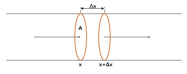
(Figure 1.2)
The concentration of component i at point x in the figure is denoted as Ci, x, and the concentration of component i at x + Δx is denoted as Ci, x+Δx. Then, let’s set up a mass(or material) balance for the volume between x and x+ Δx based on (Eq 1.1) of Mass & Heat balance Episode 01.
\( {\small\displaystyle\begin{align} i_{in} \,-\, i_{out} \,+\, i_{generation} \quad=\quad i_{accumulation} \tag{Eq 1.1 of Mass & Heat Balance} \end{align} } \)
When setting up the mass balance, we can consider the iin terms as the mass flow rate at the x position and the iout term as the mass flow rate at x+Δx. And if we assume that there is no reaction, we can rearrange the equation as follows.
\( {\small\displaystyle \begin{align} M_i A J_{i,x} \,-\, M_i A J_{i,x+Δx} \quad&=\quad {\partial m_i\over\partial x} \\[15pt] M_i A \left(D_i{\partial C_{i,x+Δx}\over\partial x}\,-\,D_i{\partial C_{i,x}\over\partial x}\right) \quad&=\quad M_i AΔx\frac{\partial C_i}{\partial t} \\[15pt] \frac{D_i}{Δx}\left({\partial C_{i,x+Δx}\over\partial x}\,-\,{\partial C_{i,x}\over\partial x}\right) \quad&=\quad \frac{\partial C_i}{\partial t},\quad Δx\,\rightarrow\,0 \tag*{} \end{align} } \)
\( {\small\displaystyle\begin{align} D_i\left({\partial^2 C_i\over\partial x^2}\right) \quad=\quad \frac{\partial C_i}{\partial t} \tag{Eq 1.5} \end{align} } \)
We refer to (Eq 1.5) as Fick’s 2nd law. We can extend this equation also to three directions. The extension for three directions can be derived by using the equation of continuity, as shown below.
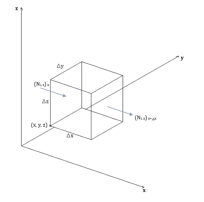
(Figure 1.3)
Assume that fluid passes through a cube as shown in (Figure 1.3). We can consider that flux flows through the 6 faces of the cube. In the figure, (Ni, x) is a vector value representing the flux moving only in the x – direction. The total value can be expressed as the sum of each vector (x, y, z – direction), and we will apply this when calculating the mass balance.
The individual terms of mass balance equation are as follows (igeneration is zero):
\( {\small\displaystyle\begin{align} i_{in} \quad&:\quad M_i \{(N_{i,x})_xΔyΔz\,+\,(N_{i,y})_yΔxΔz\,+\,(N_{i,z})_zΔxΔy\}\tag*{} \\[15pt] i_{out} \quad&:\quad M_i\{(N_{i,x})_{x+Δx}ΔyΔz\,+\,(N_{i,y})_{y+Δy}ΔxΔz\,+\,(N_{i,z})_{z+Δz}ΔxΔy\}\tag*{} \\[15pt] i_{accumulation} \quad&:\quad ΔxΔyΔzM_i\frac{\partial C_i}{\partial t}\tag*{} \end{align} } \)
After substituting the above equations into the individual terms and dividing both sides by ΔxΔyΔzMi the following equation is obtained. Then, if the values of Δx, Δy, and Δz are each infinitely close to zero, (Eq 1.6) can be derived.
\( {\small\displaystyle\begin{align} \frac{(N_{i,x})_x\,-\,(N_{i,x})_{x+∆x}}{∆x} \,+\, \frac{(N_{i,y})_y\,-\,(N_{i,y})_{y+∆y}}{∆y} \,+\, \frac{(N_{i,z})_z\,-\,(N_{i,z})_{z+∆z}}{∆z} \quad=\quad \frac{\partial C_i}{\partial t} \tag*{} \end{align} } \)
\( {\small\displaystyle\begin{align} \left(\frac{\partial (N_{i,x})_x}{\partial x}\,+\,\frac{\partial (N_{i,y})_y}{\partial y}\,+\,\frac{\partial (N_{i,z})_z}{\partial z}\right) \,+\, \frac{\partial C_i}{\partial t} \quad=\quad 0 \tag{Eq 1.6} \end{align} } \)
By (Eq 1.2), the equation can be rearranged as (Eq 1.7).
\( {\small\displaystyle\begin{gather} \left(\frac{\partial (J_{i,x}\,+\,C_iv_{0,x})}{\partial x}\,+\,\frac{\partial (J_{i,y}\,+\,C_iv_{0,y})}{\partial y}\,+\,\frac{\partial (J_{i,z}\,+\,C_iv_{0,z})}{\partial z}\right)\,+\,\frac{\partial C_i}{\partial t} \quad=\quad 0 \\[15pt] \left(\frac{\partial J_{i,x}}{\partial x}\,+\, \frac{\partial J_{i,y}}{\partial y}\,+\,\frac{\partial J_{i,z}}{\partial z}\right) \,+\,C_i\left(\frac{\partial v_{0,x}}{\partial x}\,+\,\frac{\partial v_{0,y}}{\partial y}\,+\,\frac{\partial v_{0,z}}{\partial z}\right) \,+\,v_{0,x}\frac{\partial C_i}{\partial x}\,+\,v_{0,y}\frac{\partial C_i}{\partial y}\,+\,v_{0,z}\frac{\partial C_i}{\partial z} \,+\,\frac{\partial C_i}{\partial t} \quad=\quad 0 \\[15pt] -D_i\left(\frac{\partial^2 C_i}{\partial x^2}\,+\,\frac{\partial^2 C_i}{\partial y^2}\,+\,\frac{\partial^2 C_i}{\partial z^2}\right) \,+\,C_i\left(\frac{\partial v_{0,x}}{\partial x}\,+\,\frac{\partial v_{0,y}}{\partial y}\,+\,\frac{\partial v_{0,z}}{\partial z}\right) \,+\, v_{0,x}\frac{\partial C_i}{\partial x}\,+\,v_{0,y}\frac{\partial C_i}{\partial y}\,+\,v_{0,z}\frac{\partial C_i}{\partial z} \,+\,\frac{\partial C_i}{\partial t} \quad=\quad 0\tag{Eq 1.7} \end{gather} } \)
If the average velocity(v0) of the fluid is zero, (Eq 1.7) can be simplified to (Eq 1.8), which is is an extension of Fick’s 2nd law to three directions.
\( {\small\displaystyle\begin{align} D_i\left(\frac{\partial^2 C_i}{\partial x^2}\,+\,\frac{\partial^2 C_i}{\partial y^2}\,+\,\frac{\partial^2 C_i}{\partial z^2}\right) \quad=\quad \frac{\partial C_i}{\partial t} \tag{Eq 1.8} \end{align} } \)
Nomenclature
\({\small\displaystyle A}\) : area
\({\small\displaystyle C_i}\) : mole concentration of component i
\({\small\displaystyle D_i}\) : diffusion coefficient of component i
\({\small\displaystyle J}\) : the flux of diffusion relative to the average fluid velocity
\({\small\displaystyle M}\): molecular weight
\({\small\displaystyle m}\) : mass
\({\small\displaystyle N}\) : total flux on a fixed location
\({\small\displaystyle N_i}\) : the flux of component i on a fixed location
\({\small\displaystyle t}\) : time
\({\small\displaystyle v}\) : velocity
\({\small\displaystyle v_0}\) : average velocity
\({\small\displaystyle x}\) : distance in the x – direction
\({\small\displaystyle x_i}\) : mole fraction of component i
\({\small\displaystyle y}\) : distance in the y – direction
\({\small\displaystyle z}\) : distance in the z – direction