Episode 03.
Linear Diffusion in Solids within Medium - Unsteady State
Summary
In this episode, we discuss about diffusion in a plate solid under unsteady-state conditions. We will utilize Fick’s 2nd Law, a partial differential equation. First, we analyze diffusion in a plate solid with a finite thickness within an infinite medium. And we describe diffusion in a thin film within a semi-infinite medium.
1. Introduction
In the previous episode, we described diffusion in solids under steady-state conditions, focusing on the shapes of the solid. However, we often encounter diffusion scenarios under unsteady-state conditions. Therefore, we need to calculate the diffusion under such conditions. Unsteady-state diffusion in solids is more complex compared to steady-state diffusion. So, we will cover this topic through several episodes.
As we deal with diffusion in unsteady-state conditions, we will utilize Fick’s 2nd Law, which we discussed in Episode 01. Looking at the form of Fick’s 2nd Law, we can recognize that it is a PDE (Partial Differential Equation). The PDE solutions depend on the conditions (boundary conditions, initial conditions, etc.), so it is essential to set appropriate conditions that match the specific situation.
We will discuss two representative cases concerning the diffusion from a plate solid in an infinite and semi-infinite medium.
2. Linear Diffusion in solids within an infinite medium
We assume that diffusion occurs only in the x – direction. Then, we can apply (Eq 1.5). By applying (Eq 1.5), we can recognize that concentration is a function of both “x” and “t” variables. Now, after setting the appropriate conditions for each case, we proceed to find the solutions to the partial differential equation.
\( {\small\displaystyle\begin{align} \frac{\partial C}{\partial t}\quad=\quad D\left(\frac{\partial^2 C}{\partial x^2}\right) \tag{Eq 1.5} \end{align} } \)
First, we consider a scenario where a component of a plate solid diffuses infinitely in both directions. In (Figure 3.1), there is a plate solid of thickness 2L immersed in a solution. Let’s find the solution to (Eq 1.5) when the initial concentration of the solid is uniformly C0, and the initial concentration of the solution is zero. The component moves solely by diffusion, and the diffusion coefficient remains constant.
We can express the above conditions in equations as follows, and when visualized graphically, it takes the form of (Figure 3.2).
\( {\small\displaystyle \begin{align} C \quad&=\quad f(x,t) \\[15pt] ICs \quad:\quad f(x,0)&= \begin{cases} C_0, &\mbox{for }|x|\,<\,L \\ 0, &\mbox{for } |x|\,>\,L \end{cases} \tag*{} \end{align} } \)
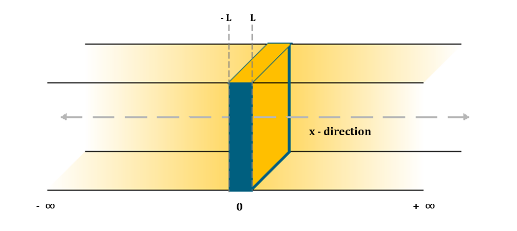
(Figure 3.1)
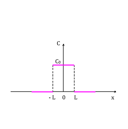
(Figure 3.2)
As the distance becomes infinitely far, we can imagine that the concentration will converge to zero. Hence, we can utilize Fourier transforms to solve the partial differential equation. Let’s apply Fourier transform to both sides of (Eq 1.5). Now, by going through the derivation steps 1 to 3, we can obtain the solution for (Eq 3.1).
\( {\small\displaystyle\begin{align}\mathcal{F}\left[\frac{\partial C}{\partial t}\right] \quad=\quad D\mathcal{F}\left[\frac{\partial^2 C}{\partial x^2}\right] \tag{Eq 3.1} \end{align} } \)
| Step 1 : Fourier transform | ||||
|---|---|---|---|---|
| From (Eq 3.1) | \( {\small\displaystyle\begin{align}\frac{\partial}{\partial t}\mathcal{F}[C]\quad=\quad -Dw^2\mathcal{F}[C]\end{align}}\) | \( {\small\longrightarrow} \) | \({\small\displaystyle\begin{align}\frac{\partial U}{\partial t}\,+\,Dw^2U \quad=\quad 0 \end{align} } \) | \( {\small\displaystyle \mathcal{F}[C]\,=\,U(w,t) } \) |
| Step 2: Solve ODE | ||||
| Laplace transform | \({\small\displaystyle\begin{align} L\left[\frac{dU}{dt}\right]\,+\,L\left[Dw^2U \right]\quad=\quad 0\end{align}}\) | \( {\small\longrightarrow} \) | \( {\small\displaystyle\begin{align} sV\,-\,U(w,0)\,+\,Dw^2V \quad=\quad 0 \end{align}} \) | \( {\small\displaystyle L[U] \,=\, V } \) |
| \( {\small\displaystyle\begin{align} V \quad=\quad \frac{\phi(w)}{s\,+\,Dw^2} \end{align} }\) | \( {\small\displaystyle\begin{align} U(w,0) \,=\, \phi(w) \end{align} }\) | |||
| Inverse laplace transform | \({\small\displaystyle\begin{align} L^{-1}[V] \quad=\quad L^{-1}\left[\frac{\phi(w)}{s\,+\,Dw^2}\right] \end{align} } \) | \( {\small\longrightarrow} \) | \( {\small\displaystyle\begin{align} U \quad=\quad \phi(w)\cdot e^{-Dw^2t} \end{align} } \) | |
| Step 3: Inverse fourier transform | ||||
| \( {\small\displaystyle\begin{align} \mathcal{F}^{-1}[U] \quad=\quad \mathcal{F}^{-1}\left[\phi(w)\cdot e^{-Dw^2t}\right] \end{align} } \) | \( {\small\longrightarrow} \) | \( {\small\displaystyle\begin{align} C \quad=\quad f(x,0) *\frac{1}{\sqrt{2Dt}}\cdot\exp\left(-\frac{x^2}{4Dt}\right) \end{align} } \) | ||
| \( {\small\displaystyle\begin{align} C \quad=\quad \frac{1}{2\sqrt{\pi Dt}}\int^{\infty}_{-\infty}f(\xi)\cdot \exp\left[{-\frac{(x\,-\,\xi)^2}{4Dt}}\right]\,d\xi \end{align} } \) | \( {\small\displaystyle *\text{: convolution} } \) |
\( {\small\displaystyle\begin{align} C(x,t) \quad=\quad \frac{1}{2\sqrt{\pi Dt}}\int^{\infty}_{-\infty}f(\xi)\cdot \exp\left[{-\frac{(x\,-\,\xi)^2}{4Dt}}\right]\,d\xi \tag{Eq 3.2} \end{align} } \)
Applying the initial conditions to (Eq 3.2) within the range of -L to L, we can express it as follows.
\( {\small\displaystyle\begin{align} C(x,t) \quad=\quad \frac{C_0}{2\sqrt{\pi Dt}}\int_{-L}^L \exp\left[\frac{-(x-\xi)^2}{2\sqrt{Dt}}\right]\,d\xi \tag{Eq 3.3} \end{align} } \)
To simplify the equation further, let’s define a new variable α.
\( {\small\displaystyle\begin{align} \frac{x\,-\,\xi}{2\sqrt{Dt}} \quad=\quad \alpha \quad\longrightarrow\quad d\xi \quad=\quad -2\sqrt{Dt}\,d\alpha \tag*{} \end{align} } \)
By rearranging (Eq 3.3) with the newly defined variable α, we obtain (Eq 3.4). Additionally, we can represent (Eq 3.4) in the form of an error function by dividing its interval with respect to x = 0.
\( {\small\displaystyle\begin{align} C \quad=\quad \frac{C_0}{\sqrt{\pi}}{\large\int}_{\tfrac{-(L+x)}{2\sqrt{Dt}}}^{\tfrac{L-x}{2\sqrt{Dt}}} \exp(-\alpha^2)\,d\alpha \tag{Eq 3.4} \end{align} } \)
\( {\small\displaystyle\begin{align} C \quad&=\quad \frac{C_0}{\sqrt{\pi}} \left[\int_0^{\tfrac{L-x}{2\sqrt{Dt}}}\exp(-\alpha^2)\,d\alpha \,+\, \int_{\tfrac{-(L+x)}{2\sqrt{Dt}}}^0 \exp(-\alpha^2)\,d\alpha \right] \\[15pt] &=\quad \frac{C_0}{2} \left[ \frac{2}{\sqrt{\pi}}\int_0^{\tfrac{L-x}{2\sqrt{Dt}}}\exp(-\alpha^2)\,d\alpha \,+\, \frac{2}{\sqrt{\pi}}\int_0^{\tfrac{L+x}{2\sqrt{Dt}}} \exp(-\alpha^2)\,d\alpha \right] \\[15pt] C(x,t) \quad&=\quad \frac{C_0}{2} \left[ erf\left(\frac{L\,-\,x}{2\sqrt{Dt}}\right) \,+\, erf\left(\frac{L\,+\,x}{2\sqrt{Dt}}\right) \right] \tag{Eq 3.5} \end{align} } \)
If we represent (Eq 3.5) graphically, how would it look? Let’s set the initial concentration, thickness, and diffusion coefficient as follows:
\( {\small\displaystyle\begin{align} C_0 \quad=\quad 10, \qquad L \quad=\quad 1, \qquad D \quad=\quad 0.025 \tag*{} \end{align} } \)
Upon substituting these values into (Eq 3.5) and representing them graphically, we get the result as shown in (Figure 3.3).
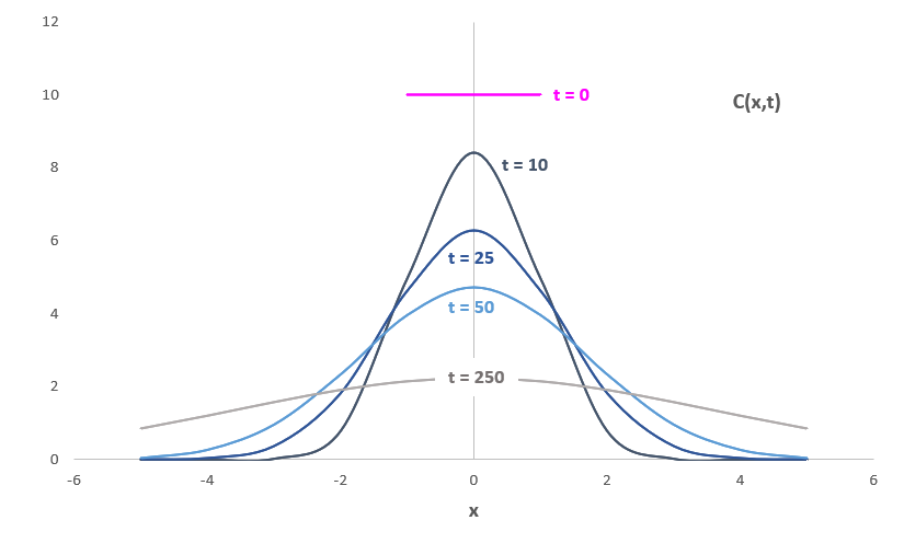
(Figure 3.3)
3. Linear diffusion in solids within a semi-infinite medium
What about the case of diffusion in semi-infinite? Let’s take a look at (Figure 3.4). In this scenario, the concentration remains constant in the region where x < 0, regrardless of time. And the component diffuses in the positive direction, away from the thin film.
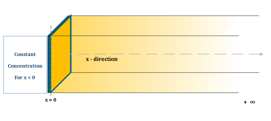
(Figure 3.4)

(Figure 3.5)
Since the range is semi-infinite(0 < x < ∞) and we know the value at x=0, we can apply the Fourier sine transform to (Eq 1.5).
\( {\small\displaystyle\begin{align} \mathcal{F}_s \left[\frac{\partial C}{\partial t}\right] \quad=\quad D\mathcal{F}_s \left[\frac{\partial^2 C}{\partial x^2}\right] \tag{Eq 3.6} \end{align} } \)
| Step 1: Fourier sine transform | ||||
|---|---|---|---|---|
| From (Eq 3.6) | \( {\small\displaystyle \frac{\partial \mathcal{F}_s[C]}{\partial t} \quad=\quad D\left[\frac{2}{\pi}wC(0)\,-\,w^2\mathcal{F}_s[C]\right] } \) | \( {\small\longrightarrow } \) | \( {\small\displaystyle \frac{\partial U}{\partial t}\,+\,Dw^2U \quad=\quad \frac{2wDC_0}{\pi} } \) | \( {\small\displaystyle \mathcal{F}_s[C] \,=\, U, \quad C(0) \,=\,C_0 } \) |
| Step 2: Solve ODE | ||||
| Laplace transform | \( {\small\displaystyle L\left[\frac{dU}{dt}\right] \,+\, L\left[Dw^2U\right] \quad=\quad L\left[\frac{2wDC_0}{\pi}\right] } \) | \( {\small\longrightarrow } \) | \( {\small\displaystyle sV\,-\,U(0)\,+\,Dw^2V \quad=\quad \frac{2wDC_0}{\pi s} } \) | \( {\small\displaystyle L[U] \,=\,V } \) |
| \( {\small\displaystyle V \quad=\quad \frac{2C_0}{\pi w} \cdot \left(\frac{1}{s}\,-\,\frac{1}{s\,+\,Dw^2}\right) } \) | \( {\small\displaystyle U(0)\,=\,0 } \) | |||
| Inverse laplace transform | \( {\small\displaystyle L^{-1}[V] \quad=\quad \frac{2C_0}{\pi w} L^{-1}\left[\frac{1}{s}\,-\,\frac{1}{s\,+\,Dw^2}\right] } \) | \( {\small\longrightarrow } \) | \( U \quad=\quad \frac{2C_0}{\pi w} \cdot \left(1\,-\,e^{-Dw^2t}\right) \) | |
| Step 3: Inverse fourier sine transform | ||||
| \( {\small\displaystyle \mathcal{F}_s^{-1}[U] \quad=\quad \mathcal{F}_s^{-1}\left[\frac{2C_0}{\pi w} \cdot \left(1\,-\,e^{-Dw^2t}\right)\right] } \) | \( {\small\longrightarrow } \) | \( {\small\displaystyle C(x,t) \quad=\quad C_0erfc\left(\frac{x}{2\sqrt{Dt}}\right) } \) | \( {\small\displaystyle erfc(x)\,=\,1\,-\,erf(x) } \) |
\( {\small\displaystyle\begin{align} C(x,t) \quad=\quad C_0erfc\left(\frac{x}{2\sqrt{Dt}}\right) \tag{Eq 3.7} \end{align} } \)
When we plot (Eq 3.7), it takes the graph shown below. (C0 = 10, D = 0.025)
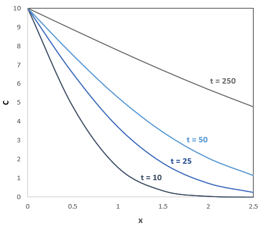
(Figure 3.6)
As previously mentioned, since PDEs depend on the given conditions, the solutions derived in this episode do not fully cover all diffusion scenarios from a plate solid in an infinite or semi-infinite medium. However, approaching various cases by setting suitable conditions as we discussed in this episode, you can derive solutions for diffusion in each scenario.
Nomenclature
\({\small\displaystyle C}\) : concentration
\({\small\displaystyle D}\) : diffuision coefficient
\({\small\displaystyle erf}\) : error function
\({\small\displaystyle \text{PDE}}\) : partial differential equation
\({\small\displaystyle t}\) : time
\({\small\displaystyle w,x}\) : variable
\(\small\displaystyle\mathcal{F}\) : fourier transform
\(\small\displaystyle\mathcal{F}_s\) : fourier sine transform