Episode 05. Control Valve Sizing Method
Summary
Selecting an appropriate-sized valve is essential to achieve the desired flow rate. In this episode, we discuss how to size control valves based on the phase of the fluid.
1. Introduction
As mentioned in Episode 03, we must select the appropriate valve size even after choosing its type. For on/off valves, we match the size to the connected pipe. However, control valves are different. Too small a valve may not produce the desired flow rate, while too large a valve can increase costs and make precise control difficult. So, how should we determine the appropriate size? In this episode, we introduce how to select the size of a control valve. We need to know the required \({\small\displaystyle C(C_v}\)or \({\small\displaystyle K_v)}\) to choose the size. And how we calculate the \({\small\displaystyle C}\) depends on the phase of the fluid passing through the valve.
2. Sizing control valve for liquid service
Now, let’s look at how to select the size of control valves for liquid service. We can calculate the required \({\small\displaystyle C}\) for a liquid to pass through a valve using (Eq 5.1). In this equation, \({\small\displaystyle F_p}\) is the piping geometry factor, which accounts for the effects of fittings installed upstream and downstream of the valve. \({\small\displaystyle \Delta P_a}\) represents the actual pressure drop across the valve.
\( {\small\displaystyle\begin{align} C(C_v\,\text{or}\,K_v) \quad=\quad \frac{Q}{F_p} \times \sqrt{\frac{S_g}{\Delta P_a}} \tag{Eq 5.1} \end{align} } \)
Before calculating the \({\small\displaystyle C}\) using (Eq 5.1), it is necessary to check several factors. The first is to determine whether there is a phase change. We can distinguish it by comparing the pressure profile in the valve with the fluid vapor pressure.
Typically, the velocity increases, and the pressure decreases as the valve’s diameter narrows. The pressure becomes lowest at the vena contracta and later recovers as the valve’s area increases from the vena contracta to the outlet. We can broadly classify the phase changes into three cases in this process. Refer to (Figure 5.1) for details. \({\small\displaystyle P^v}\) refers to the vapor pressure of the liquid, \({\small\displaystyle P_1}\) is the pressure at the valve inlet, \({\small\displaystyle P_2}\) is the pressure at the valve outlet, and \({\small\displaystyle P_{vc}}\) is the pressure at the vena contracta.
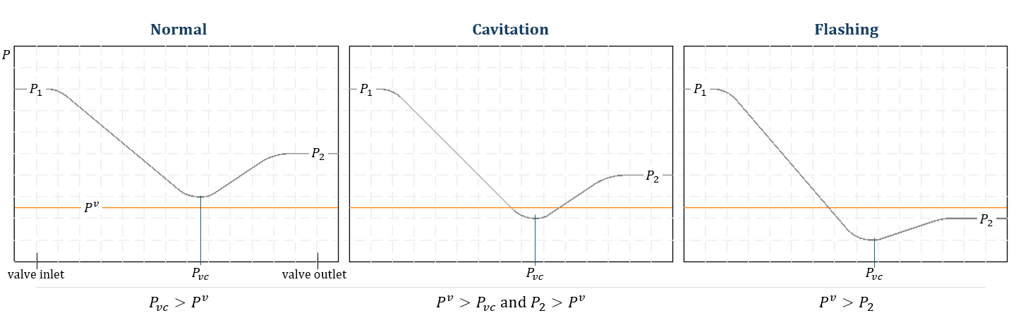
(Figure 5.1)
The first case is when \({\small\displaystyle P_{vc}}\) is greater than the \({\small\displaystyle P^v}\), in which case no phase change occurs. The second case is when \({\small\displaystyle P_{vc}}\) is lower than the \({\small\displaystyle P^v}\), but \({\small\displaystyle P_2}\) is higher than the \({\small\displaystyle P^v}\). In this case, the fluid undergoes a phase change from liquid to vapor and back to liquid, resulting in cavitation. Cavitation can cause damage to the valve, potentially requiring changes to the valve’s component material. The final case is when \({\small\displaystyle P_2}\) is lower than \({\small\displaystyle P^v}\), leading to a phase change from liquid to vapor and resulting in flashing. Since vapor has a much larger volume compared to liquid, in this case, it’s important to check the velocity at the outlet.
\( {\small\displaystyle P_2\quad > \quad P^v } \)
If \({\small\displaystyle P_2}\) is greater than \({\small\displaystyle P^v}\), we should check whether the fluid passing through the valve becomes a choked flow. Typically, as the downstream pressure decreases (i.e., the pressure drop across the valve increases), the fluid velocity increases.

(Figure 5.2)
However, when the downstream pressure falls below a certain point, the velocity stops increasing, and this phenomenon is called choked flow. So why does choked flow occur?
As mentioned earlier, the liquid passing through the valve can change into vapor under certain conditions. When the fluid vaporizes, its volume rapidly expands, and the velocity can reach the speed of sound. Since the fluid cannot exceed the speed of sound by simply lowering the downstream pressure, the pressure drop that causes choked flow becomes the maximum pressure differential. (Figure 5.2) shows a graph about the flow rate against the pressure drop.
We can calculate the differential pressure at which choked flow occurs using (Eq 5.2). In (Eq 5.2), \({\small\displaystyle F_L}\) is the pressure recovery factor, which can be calculated using (Eq 5.3). However, since \({\small\displaystyle P_{vc}}\) varies depending on the type and shape of the valve, it is most accurate to check this from the manufacturer. \({\small\displaystyle F_F}\) is the liquid-critical pressure ratio factor, which can be obtained using (Eq 5.4).
\( {\small\displaystyle\begin{align} \Delta P_{choked} \quad&=\quad F_L^2\left(P_1\,-\,F_FP^v\right) \tag{Eq 5.2} \\[15pt] F_L \quad&=\quad \sqrt{\frac{P_1\,-\,P_2}{P_1\,-\,P_{vc}}} \tag{Eq 5.3} \\[15pt] F_F \quad&=\quad 0.96\,-\,0.28\sqrt{\frac{P^v}{P_c}} \tag{Eq 5.4} \end{align} } \)
\({\small\displaystyle F_L}\) is the value when the valve is alone. We use \({\small\displaystyle F_{LP}/F_P}\) instead of \({\small\displaystyle F_L}\) when attaching fittings to the valve. We can calculate \({\small\displaystyle F_{LP}}\) using (Eq 5.6), though it is an estimate and may have some error.
\( {\small\displaystyle\begin{align} \Delta P_{choked} \quad&=\quad \left(\frac{F_{LP}}{F_P}\right)^2\left(P_1\,-\,F_FP^v\right) \tag{Eq 5.5} \\[15pt] F_{LP} \quad&=\quad \frac{F_L}{\sqrt{1\,+\,\dfrac{F_L^2\sum\xi_i}{N_2}\left(\dfrac{C}{d_{nom}^2}\right)^2}} \tag{Eq 5.6} \\[10pt] \text{where}\quad \\[10pt] \sum\xi_i \quad&=\quad \xi_1\,+\,\xi_{B1} \\[10pt] \xi_{1} \quad&=\quad \text{inlet fitting resistance coefficient} \\[10pt] \xi_{B1} \quad&=\quad 1\,-\,\left(d_{nom}/d_1\right)^4,\,\text{inlet Bernoulli coefficient} \end{align} } \)
The pressure difference at which choked flow occurs is the maximum allowable pressure drop. Therefore, if \({\small\displaystyle P_1\,-\,P_2}\) exceeds \({\small\displaystyle \Delta P_{choked}}\), the \({\small\displaystyle \Delta P_a}\) in (Eq 5.1) becomes \({\small\displaystyle \Delta P_{choked}}\).
Next, we need to check whether the flow through the valve is laminar or turbulent. To do this, we calculate the Reynolds number as the flow passes through the valve. The valve Reynolds number,\({\small\displaystyle Re_v}\), is:
\( {\small\displaystyle\begin{align} Re_v \quad=\quad \frac{N_4F_dQ}{\upsilon\sqrt{F_LC}}\left(\frac{F_L^2C^2}{N_2d^4}+1\right)^{0.25} \tag{Eq 5.7} \end{align} } \)
\({\small\displaystyle F_d}\) is a valve style modifier that varies depending on the valve and trim type. \({\small\displaystyle N}\) represents numerical constants, and its value depends on the units used. We can find both values in the ANSI/ISA-75.01.01 standard. For \({\small\displaystyle F_d}\), typical values can be obtained from the document, but the values provided by the manufacturer are more accurate. We use the \({\small\displaystyle Re_v}\) obtained from (Eq 5.7) for calculating the Reynolds number factor, \({\small\displaystyle F_r}\).
If the \({\small\displaystyle Re_v}\) is greater than 40,000, \({\small\displaystyle F_R}\) is 1; if it is less than 40,000, it can be calculated using (Eq 5.8).
\( {\small\displaystyle\begin{align} F_R \quad&=\quad 1.044\,-\,0.358\left(\frac{C_S}{C_T}\right)^{0.655},\quad Re_v \,\le\,40,000 \tag{Eq 5.8} \\[15pt] C_S \quad&=\quad \frac{1}{F_S}\left(\frac{Q\mu}{N_s\Delta P_a}\right)^{2/3}\quad \begin{cases} N_s\,=\,47 & Q[\text{gpm}],\,\Delta P[\text{psi}] \\[10pt] N_s\,=\,15 & Q[\text{m}^3\text{/hr}],\,\Delta P[\text{bar}] \end{cases} \tag{Eq 5.9} \\[15pt] F_S \quad&=\quad \frac{F_d^{2/3}}{F_L^{1/3}}\left(\frac{F_L^2C^2}{N_2d^4}\,+\,1\right)^{1/6} \tag{Eq 5.10} \end{align} } \)
Then, we calibrate the flow coefficient value depending on the range over which \({\small\displaystyle F_R}\) lies.
\( {\small\displaystyle\begin{align} \begin{cases} C \quad=\quad C_S &F_R\,<\,0.48 \\[10pt] C \quad=\quad \dfrac{Q}{F_R}\sqrt{\dfrac{S_g}{\Delta P_a}} &0.48\,<\,F_R\,<\,0.98 \\[10pt] C \quad=\quad C_T\,(\text{Eq 5.1}) &F_R\,>\,0.98 \tag{Eq 5.11} \end{cases} \end{align} } \)
Finally, determine the required \({\small\displaystyle C}\) value by applying the \({\small\displaystyle F_p}\) factor.
\( {\small\displaystyle\begin{align} F_p \quad&=\quad \frac{1}{\sqrt{1\,+\,\dfrac{\sum\xi}{N_2}\left(\dfrac{C}{d_{nom}^2}\right)^2}} \tag{Eq 5.12} \\[10pt] \text{where}\quad \\[10pt] \sum\xi \quad&=\quad \xi_1\,_\,+\,\xi_2\,+\,\xi_{B1}\,-\,\xi_{B2} \\[10pt] \xi_{1,2} \quad&=\quad \text{fitting resistance coefficient} \\[10pt] \xi_{B1} \quad&=\quad 1\,-\,\left(d_{nom}/d_1\right)^4,\,\text{inlet Bernoulli coefficient} \\[10pt] \xi_{B2} \quad&=\quad 1\,-\,\left(d_{nom}/d_2\right)^4,\,\text{outlet Bernoulli coefficient} \end{align} } \)
\( {\small\displaystyle P^v\quad > \quad P_2 } \)
In this case, both liquid and gas phases are present, so the ratio of liquid and gas at the outlet is important. If we define the gas ratio as \({\small\displaystyle x}\), we can calculate the volumetric flow rate as follows.
\( {\small\displaystyle\begin{align} Q \quad=\quad w\left[(1\,-\,x)\hat{V_{2l}}\,+\,x\hat{V_{2g}}\right] \tag{Eq 5.13} \end{align} } \)
We can obtain the gas ratio \({\small\displaystyle x}\) through material (mass) and energy (heat) balances. (Please refer to the Mass & Heat Balance content.)
\( {\small\displaystyle\begin{align} x \quad=\quad \frac{\Delta H_{1l}\,-\,\Delta H_{2l}}{\Delta H_{e}} \tag{Eq 5.14} \end{align} } \)
Calculate the outlet velocity based on the equations and evaluate its suitability. If the velocity is too high and could damage the valve, we should adjust the material and size.
3. Sizing control valve for gas service
Now, let’s discuss how to size a control valve for gas flow. Gas is a compressible fluid, so its volumetric flow rate varies with pressure. To consider this, we use a coefficient called the expansion factor \({\small\displaystyle Y}\).
\( {\small\displaystyle\begin{align} Y \quad&=\quad 1\,-\,\frac{x}{3F_{\gamma}x_T} \tag{Eq 5.15} \\[15pt] x \quad&=\quad \frac{\Delta P_a}{P_1} \tag{Eq 5.16} \\[15pt] F_{\gamma} \quad&=\quad \frac{\gamma}{1.4},\,\gamma\,=\,C_P/C_V \tag{Eq 5.17} \end{align} } \)
\({\small\displaystyle F_\gamma}\) is the ratio of specific heats factor. The terminal pressure drop ratio, \({\small\displaystyle x_T}\), varies depending on the type of valve. We can find the typical value of \({\small\displaystyle x_T}\) in ANSI/ISA-75.01.01 standard.
\({\small\displaystyle x_T}\)’s value is based on the valve alone, so it should be replaced with \({\small\displaystyle x_{TP}}\) for the calculations when attaching fittings.
\( {\small\displaystyle\begin{align} x_{TP} \quad&=\quad \frac{x_T}{F_P^2\left[1\,+\,\dfrac{x_T\sum\xi_i}{N_5}\left(\dfrac{C}{d_{nom}}\right)^2\right]} \tag{Eq 5.18} \end{align} } \)
If \({\small\displaystyle x}\) exceeds \({\small\displaystyle F_\gamma x_{T}}\)(or \({\small\displaystyle F_\gamma x_{TP}}\)), choked flow occurs. Therfore, the minimum possible value of the expansion factor is 2/3.
Based on (Eq 5.1), after rearranging with \({\small\displaystyle Q}\) on the left side and the remaining terms on the right side and applying \({\small\displaystyle Y}\), we can express it as follows.
\( {\small\displaystyle\begin{align} Q \quad=\quad CF_pY\sqrt{\frac{\Delta P_a}{S_g}} \tag{Eq 5.19} \end{align} } \)
We can rearrange (Eq 5.19) for various unit bases.
\( {\small\displaystyle\begin{align} w\,[\text{kg/hr}] \quad&=\quad 31.6K_vF_pY\sqrt{xP_1\rho_1} \\ \tag{Eq 5.20} \\ w\,[\text{lb/hr}] \quad&=\quad 63.3C_vF_pY\sqrt{xP_1\rho_1} \\[15pt] Q_s\,[\text{m}^3/\text{hr}] \quad&=\quad 2458K_vF_PP_1Y\sqrt{\dfrac{x}{Z_1T_1M_w}} \\ \tag{Eq 5.21} \\ Q_s\,[\text{scfh}] \quad&=\quad 6939C_vF_PP_1Y\sqrt{\dfrac{x}{Z_1T_1M_w}} \end{align} } \)
We apply the appropriate equations from above based on the given conditions. \({\small\displaystyle Q_s}\) is the value based on the gas standard conditions (\({\small\displaystyle 0^{\circ}\text{C},\,\text{1 atm}}\)).
And we should consider the outlet velocity from the valve in the gas service. When evaluating the velocity of gas, we can gauge it relative to the Mach number.
\( {\small\displaystyle\begin{align} Ma \,=\, \frac{u}{a},\quad a\,=\, \sqrt{\left(\frac{dP}{d\rho}\right)_s},\quad P\,=\, \frac{R}{M_w}\rho T \tag*{} \end{align} } \)
The speed of sound is an adiabatic, or isentropic, process. The isentropic process satisfies the following relationships.
\( {\small\displaystyle\begin{align} P\rho^{-\gamma} \,=\, \text{constant} \quad&\longrightarrow\quad \ln P\,-\,\gamma\ln\rho \,=\, \text{constant} \\[10pt] \frac{dP}{P}\,-\,\gamma\frac{d\rho}{\rho} \,=\,0 \quad&\longrightarrow\quad \frac{dP}{d\rho} \,=\, \gamma\frac{P}{\rho} \tag*{} \end{align} } \)
Therefore, we can express the Mach number as follows.
\( {\small\displaystyle\begin{align} Ma \quad&=\quad \frac{Q}{A_v\sqrt{\gamma TR/M_w}},\quad \\ \tag{Eq 5.22} \\ Ma \quad&=\quad \frac{Q}{0.186A_v\sqrt{\gamma TR/G_g}} \end{align} } \)
If the Mach number exceeds 0.5, vibrations and noise can occur. So, we should take precautions in this case. If the outlet velocity’s Mach number is greater than 1, we should change the valve size.
Nomenclature
\({\small\displaystyle a}\) : speed of sound
\({\small\displaystyle C,\,C_v,\,K_v}\) : flow coefficients
\({\small\displaystyle d_{nom}}\) : nominar diameter
\({\small\displaystyle F_F}\) : liquid-critical pressure ratio factor
\({\small\displaystyle F_L}\) : pressure recovery factor without attached fittings
\({\small\displaystyle F_{LP}}\) : pressure recovery factor with attached fittings
\({\small\displaystyle F_P}\) : piping geometry factor
\({\small\displaystyle F_R}\) : Reynolds number factor
\({\small\displaystyle G_g}\) : gas specific gravity
\({\small\displaystyle H}\) : enthalpy
\({\small\displaystyle M_w}\) : molecular weight
\({\small\displaystyle P}\) : pressure
\({\small\displaystyle P^v}\) : vapor pressure
\({\small\displaystyle P_{vc}}\) : pressure at a vena contracta
\({\small\displaystyle \Delta P_a}\) : actual pressure drop
\({\small\displaystyle Q}\) : volumetric flow rate
\({\small\displaystyle R}\) : gas constant
\({\small\displaystyle S_g}\) : specific gravity
\({\small\displaystyle T}\) : temperature
\({\small\displaystyle \hat{V}}\) : specific volume
\({\small\displaystyle v}\) : velocity
\({\small\displaystyle w}\) : mass flow rate
\({\small\displaystyle x}\) : gas ratio
\({\small\displaystyle Y}\) : expansion factor
\({\small\displaystyle Z}\) : compressibility factor
\({\small\displaystyle \gamma}\) : ratio of specific heats
\({\small\displaystyle \rho}\) : density
\({\small\displaystyle \rho_w}\) : density of water
\({\small\displaystyle \xi}\) : resistance coefficient