
Episode 03. Conduction - Unsteady State
Summary
The temperature of an object does not necessarily remain constant during heat conduction. In this episode, we focus on the mathmatical modeling of conduction under unsteady state. Using partial differential equations (PDEs) in various coordinate systems- Cartesian, cylindrical, and spherical-we discuss how the temperature of an object changes over time.
1. Introduction
While the previous episode focused on steady-state heat conduction, where temperature remains constant over time, this episode explores unsteady-state conduction. We use partial differential equations (PDEs) for conduction to analyze how temperature varies over time under given initial and boundary conditions. The PDEs for conduction in different coordinate systems are:
\( {\small\displaystyle\begin{align} \text{Cartesian :}\quad \frac{dT}{dt} \quad&=\quad \alpha \left(\frac{\partial^2T}{\partial x^2}\,+\,\frac{\partial^2T}{\partial y^2}\,+\,\frac{\partial^2T}{\partial z^2}\right) \tag*{} \\[15pt] \text{Cylindrical :}\quad \frac{\partial T}{\partial t} \quad&=\quad \frac{\alpha}{r} \left[\frac{\partial}{\partial r} \left(r\frac{\partial T}{\partial r}\right) \,+\, \frac{\partial}{\partial\theta} \left(\frac{1}{r}\frac{\partial T}{\partial\theta}\right) \,+\, \frac{\partial}{\partial z} \left(r\frac{\partial T}{\partial z}\right) \right] \\[15pt] \text{Sphreical :}\quad \frac{\partial T}{\partial t} \quad&=\quad \frac{\alpha}{r^2} \left[ \frac{\partial}{\partial r} \left(r^2\frac{\partial T}{\partial r} \right) \,+\, \frac{1}{\sin\theta}\frac{\partial}{\partial\theta} \left(\sin\theta\frac{\partial T}{\partial\theta}\right) \,+\, \frac{1}{\sin^2\theta}\frac{\partial^2T}{\partial\phi^2} \right] \end{align} } \)
2. Unsteady-state conduction in varous coordinate systems
Let’s formulate a mathematical model for how temperature changes for conduction based on each PDE.

(Figure 3.1)
Conduction in plates
Consider a plate with a thickness of \({\small\displaystyle 2L}\), as shown in (Figure 3.1). The surfaces at \({\small\displaystyle x\,=\,0}\) and \({\small\displaystyle x\,=\,2L}\) are maintained at a constant temperature \({\small\displaystyle T_s}\), and the plate is initially at a uniform temperature \({\small\displaystyle T_0}\). Heat transfer occurs only by conduction in the x-direction.
\( {\small\displaystyle\begin{align} \frac{dT}{dt} \quad&=\quad \alpha \frac{\partial^2T}{\partial x^2} \tag{Eq 3.1} \\[10pt] T(x,0) \quad&=\quad T_0 \\[10pt] T(0,t) \quad&=\quad T_s,\qquad T(2L,t) \quad=\quad T_s \end{align} } \)
The solution to this PDE follows from (Eq 4.4) as introduced in Episode 04 under the Mass Transfer category. So,
\( {\small\displaystyle\begin{align} T(x,t) \quad=\quad T_s \,+\, \frac{2}{\pi} \sum_{n=1}^{\infty} &\frac{T_s\{\cos(n\pi)\,-\,1\}}{n} \exp\left[-\alpha\left(\frac{n\pi}{2L}\right)^2t\right]\sin\left(\frac{n\pi}{2L}x\right) \\ \tag{Eq 3.2} \\ &\,+\, \frac{1}{L} \sum_{n=1}^{\infty} \exp\left[-\alpha\left(\frac{n\pi}{2L}\right)^2t\right]\sin\left(\frac{n\pi}{2L}x\right) \int_0^{2L}\,T_0\sin\left(\frac{n\pi}{2L}x'\right)\,dx' \end{align} } \)
And rearranging (Eq 3.2) yields the following expression:
\( {\small\displaystyle\begin{align} T(x,t) \quad&=\quad T_s \,+\, \frac{2}{\pi} \sum_{n=1}^{\infty} \frac{T_s\{\cos(n\pi)\,-\,1\}}{n} \exp\left[-\alpha\left(\frac{n\pi}{2L}\right)^2t\right]\sin\left(\frac{n\pi}{2L}x\right) \\ \tag{Eq 3.3} \\ &\qquad\qquad\qquad\,-\, \frac{2}{\pi} \sum_{n=1}^{\infty} \exp\left[-\alpha\left(\frac{n\pi}{2L}\right)^2t\right]\sin\left(\frac{n\pi}{2L}x\right) \frac{T_0\{\cos(n\pi)\,-\,1\}}{n} \\[15pt] &=\quad T_s \,+\, \frac{2}{\pi} \sum_{n=1}^{\infty} \frac{T_s\{\cos(n\pi)\,-\,1\}}{n} \exp\left[-\alpha\left(\frac{n\pi}{2L}\right)^2t\right]\sin\left(\frac{n\pi}{2L}x\right) (T_s\,-\,T_0) \tag{Eq 3.4} \end{align} } \)
An alternative expression for the temperature is as follows.
\( {\small\displaystyle\begin{align} \frac{T_s\,-\,T_0}{T_s\,-\,T_0} \quad&=\quad \frac{\dfrac{2}{\pi}\displaystyle\sum_{n=1}^{\infty}\dfrac{\{1\,-\,\cos(n\pi)\}}{n}\exp\left[-\alpha\left(\frac{n\pi}{2L}\right)^2t\right]\sin\left(\dfrac{n\pi}{2L}x\right)(T_s\,-\,T_0)}{T_s\,-\,T_0} \tag{Eq 3.5} \\[15pt] &=\quad \frac{4}{\pi} \left[e^{-\pi^2F_o/4}\sin\left(\frac{\pi}{2L}x\right)\,+\, e^{-9\pi^2F_o/4}\sin\left(\frac{3\pi}{2L}x\right)\,+\, e^{-25\pi^2F_o/4}\sin\left(\frac{5\pi}{2L}x\right)\,+\, \cdots \right] \tag{Eq 3.6} \\[10pt] &\quad\text{where }\quad F_o\,=\, \frac{\alpha t}{L^2} \end{align} } \)
While (Eq 3.5) and (Eq 3.6) provide the local temperature within the plate, how can we determine the average temperature across the plate? Assume \({\small\displaystyle \bar{T}}\) is mean temperature. Then,
\( {\small\displaystyle\begin{align} \frac{T_s\,-\,\bar{T}}{T_s\,-\,T_0} \quad&=\quad \frac{1}{2L}\int_{0}^{2L}\,\frac{T_s\,-\,T}{T_s\,-\,T_0}\,dx \tag{Eq 3.7} \\[15pt] &=\quad \frac{8}{\pi^2} \left[\exp\left(-\frac{\pi^2F_o}{4}\right)\,+\,\frac{1}{9}\exp\left(-\frac{9\pi^2F_o}{4}\right)\,+\,\frac{1}{25}\exp\left(-\frac{25\pi^2F_o}{4}\right)\,+\,\cdots\right] \tag{Eq 3.8} \end{align} } \)
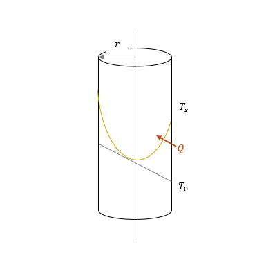
(Figure 3.2)
Conduction in cylinder
Now, let us examine heat conduction in cylindrical coordinates. Assuming that heat transfer occurs only in the radial direction, the PDE for unsteady state is as follows.
\( {\small\displaystyle\begin{align} \frac{dT}{dt} \quad&=\quad \alpha\left(\frac{1}{r}\frac{\partial T}{\partial r}\,+\,\frac{\partial^2T}{\partial r^2}\right) \tag{Eq 3.9} \\[10pt] T(a,t) \quad&=\quad T_s \\[10pt] T(r,0) \quad&=\quad T_0 \end{align} } \)
A detailed solution procedure for the above PDE can be found in Episode 05 of the Mass Transfer category.
\( {\small\displaystyle\begin{align} T(r,t) \quad&=\quad T_s\,+\, \frac{2(T_s\,-\,T_0)}{a}\sum_{n=1}^{\infty}\frac{1}{\sigma_n}\frac{J_0(\sigma_nr)}{J_0'(\sigma_na)}\exp\left(-\alpha\sigma_n^2t\right) \tag{Eq 3.10} \\[15pt] \frac{T_s\,-\,T}{T_s\,-\,T_0} \quad&=\quad -\frac{2}{a}\sum_{n=1}^{\infty}\frac{1}{\sigma_n}\frac{J_0(\sigma_nr)}{J_0'(\sigma_na)}\exp(-\alpha\sigma_n^2t) \tag{Eq 3.11} \end{align} } \)
To determine the mean temperature of the cylinder, we can use the following equation.
\( {\small\displaystyle\begin{align} \frac{T_s\,-\,\bar{T}}{T_s\,-\,T_0} \quad&=\quad \frac{1}{\pi a^2}\int_0^a\,2\pi r \left(\frac{T_s\,-\,T}{T_s\,-\,T_0}\right)\,dr \quad=\quad \frac{2}{a^2}\int_0^a\,r\left(\frac{T_s\,-\,T}{T_s\,-\,T_0}\right)\,dr \tag{Eq 3.12} \\[15pt] &=\quad \frac{4}{a^2}\sum_{n=1}^{\infty}\frac{1}{\sigma_n^2}\exp\left(-\alpha\sigma_n^2t\right) \tag{Eq 3.13} \end{align} } \)
\({\small\displaystyle \sigma_n}\), as used in (Eq 3.13), must satisfy the following condition.
\( {\small\displaystyle\begin{gather} J_0(\sigma_na) \,=\, 0 \quad\longrightarrow\quad \sigma_1 \,=\,\frac{2.405}{a},\qquad \sigma_2 \,=\,\frac{5.520}{a},\qquad \sigma_3 \,=\,\frac{8.654}{a},\qquad \cdots \tag{Eq 3.14} \end{gather} } \)
Substituting each value of \({\small\displaystyle\sigma_n}\) into (Eq 3.13) yields an equation for the mean temperature.
\( {\small\displaystyle\begin{align} \frac{T_s\,-\,\bar{T}}{T_s\,-\,T_0} \quad&=\quad 0.692\exp(-5.78F_o)\,+\,0.131\exp(-30.5F_o)\,+\,0.0534\exp(-74.9F_o)\,+\,\cdots \tag{Eq 3.15} \\[10pt] &\quad\text{where }\quad F_o\,=\, \frac{\alpha t}{a^2} \end{align} } \)
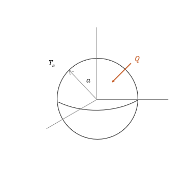
(Figure 3.2)
Conduction in spheres
Finally, we consider heat conduction in a sphere with radius \({\small\displaystyle a}\). Introducing the variable \({\small\displaystyle u}\), the corresponding PDE can be written as follows.
\( {\small\displaystyle\begin{align} u \quad&=\quad T\,\cdot\,r \\[15pt] \frac{\partial u}{\partial t} \quad&=\quad \alpha\frac{\partial^2u}{\partial r^2} \tag{Eq 3.16} \\[10pt] u(a,t) \quad&=\quad aT_S \\[10pt] u(r,0) \quad&=\quad rT_0 \end{align} } \)
The solution method for this PDE is detailed in Episode 08 of the Mass Transfer category. Applying (Eq 8.5) from that episode yields the solution.
\( {\small\displaystyle\begin{align} u \quad&=\quad rT_s\,+\, \frac{2a(T_s\,-\,T_0)}{\pi}\sum_{n=1}^{\infty} \frac{(-1)^n}{n} \sin\left(\frac{n\pi r}{a}\right) \exp\left(\frac{-\alpha n^2\pi^2t}{a^2}\right) \tag{Eq 3.17} \\[15pt] T(r,t) \quad&=\quad T_s\,+\, \frac{2a(T_s\,-\,T_0)}{\pi r}\sum_{n=1}^{\infty} \frac{(-1)^n}{n} \sin\left(\frac{n\pi r}{a}\right) \exp\left(\frac{-\alpha n^2\pi^2t}{a^2}\right) \tag{Eq 3.18} \end{align} } \)
As in the previous two cases, we can calculate the average temperature in the sphere.
\( {\small\displaystyle\begin{align} \frac{T_s\,-\,\bar{T}}{T_s\,-\,T_0} \quad&=\quad \frac{3}{4\pi a^3}\int_0^a\,4\pi r^2\frac{T_s\,-\,T}{T_s\,-\,T_0}\,dr \quad=\quad \frac{3}{a^3}\int_0^a\,r^2\frac{T_s\,-\,T}{T_s\,-\,T_0}\,dr \tag{Eq 3.19} \\[15pt] &=\quad \frac{6}{\pi^2} \sum_{n=1}^{\infty} \,\frac{\exp\left(-n^2\pi^2F_o\right)}{n^2} \tag{Eq 3.20} \\[15pt] &=\quad 0.608\exp(-9.87F_o)\,+\,0.152\exp(-39.5F_o)\,+\,0.0676\exp(-88.8F_o)\,+\,\cdots \tag{Eq 3.21} \\[10pt] &\quad\text{where }\quad F_o\,=\, \frac{\alpha t}{a^2} \end{align} } \)
(Figure 3.4) illustrates the three cases discussed above as a plot.

(Figure 3.4)
3. Internal vs External thermal resistance
From (Eq 3.2) to (Eq 3.21) assume a constant ambient temperature. However, when the surface temperature varies and external thermal resistance is present, the Biot number is introduced to represent the ratio between external and internal thermal resistance.
\( {\small\displaystyle\begin{align} \text{Bi} \quad=\quad \frac{hL}{k} \quad\text{or}\quad \frac{hr}{k} \tag{Eq 3.22} \end{align} } \)
A large Biot number indicates low external thermal resistance, allowing the surface temperature of the solid to be considered nearly constant. In such cases, (Figure 3.4) is applicable. Conversely, a small Biot number implies negligible internal resistance, meaning the entire solid can be treated as having a uniform temperature.
The average temperature of the solid can then be determined using standard charts that relate the Fourier and Biot numbers, which are commonly found in heat transfer handbooks.
Nomenclature
\({\small\displaystyle \text{Bi}}\) : Biot number
\({\small\displaystyle F_o}\) : Fourier number
\({\small\displaystyle h}\) : heat transfer coefficient
\({\small\displaystyle J}\) : Bessel function of the first kind
\({\small\displaystyle k}\) : thermal conductivity
\({\small\displaystyle L}\) : length
\({\small\displaystyle r}\) : radius
\({\small\displaystyle T}\) : temperature
\({\small\displaystyle T_o}\) : initial temperature
\({\small\displaystyle T_s}\) : surface temperature
\({\small\displaystyle \bar{T}}\) : mean temperature
\({\small\displaystyle t}\) : time
\({\small\displaystyle u}\) : variable
\({\small\displaystyle \alpha}\) : thermal diffusivity