Episode 04.
Forced Convection in Laminar Flow - No Phase Change
Summary
In this episode, we discuss forced convection under laminar flow conditions. Since there are no eddies in laminar flow, heat transfer occurs primarily through conduction. Based on this, we examine how heat transfer behaves in a circular pipe for both plug flow and thermally fully developed flow.
1. Introduction
Convection is generally classified into two categories: forced convection and natural convection. Since convection involves heat transfer through fluid motion, the characteristics of the flow are an important factor.
In this episode, we discuss forced convection in laminar flow in a pipe (or tube). Assuming no phase change, let’s explore how heat transfer occurs under various conditions. Several dimensionless numbers are commonly used in the analysis of convective heat transfer. (Table 4.1) summarizes the key dimensionless numbers.
Let’s examine the relationship between the mean temperature and the local temperature of the fluid. The total heat transfer rate is equal to the sum of heat transfer across each differential cross-sectional area. Based on this relationship, we obtain (Eq 4.1) :
\( {\small\displaystyle\begin{align} \dot{m}C_p\bar{T} \quad&=\quad \int_A\,\rho vC_pT\,dA \\[15pt] \bar{T} \quad&=\quad \frac{\int_A\,\rho vC_pT\,dA}{\rho\bar{v}C_pA} \tag{Eq 4.1} \end{align} } \)
Assuming constant density and heat capacity, and flow inside a circular pipe, this expression can be simplified to (Eq 4.2).
\( {\small\displaystyle\begin{align} \bar{T} \quad=\quad \frac{2\pi\int_0^{r_0}\,\rho vC_pTr\,dr}{\rho\bar{v}C_p\pi r_0^2} \quad=\quad \frac{2}{\bar{v}r_0^2}\int_0^{r_0}\,vTr\,dr \tag{Eq 4.2} \end{align} } \)
Now, let’s discuss forced convection under laminar flow conditions. Since there are no eddies in laminar flow, heat transfer is governed primarily by conduction. In this case, the heat transfer behavior can be further categorized depending on the flow profile. Typical cases include plug flow and fully developed flow, as shown in (Figure 4.1).
| Dimensionless Number | Name | Formula |
|---|---|---|
| \({\small\displaystyle\text{Bi}}\) | Biot number | \({\small\displaystyle\frac{hD}{k}}\) |
| \({\small\displaystyle\text{Fo}}\) | Fourier number | \({\small\displaystyle\frac{\alpha t_T}{r^2}}\) |
| \({\small\displaystyle\text{Gr}} \) | Grashof number | \({\small\displaystyle\frac{D_o^3\rho_f^2\beta g\Delta T_o}{u_f^2} }\) |
| \({\small\displaystyle\text{Gz}} \) | Graetz number | \({\small\displaystyle}\frac{\dot{m}C_p}{kL} \) |
| \({\small\displaystyle\text{Nu}} \) | Nusselt number | \({\small\displaystyle\frac{hD}{k}} \) |
| \({\small\displaystyle\text{Pe}} \) | Peclet number | \({\small\displaystyle\text{Re Pr}\left(=\frac{\rho vC_pD}{k}\right)} \) |
| \({\small\displaystyle\text{Pr}} \) | Prandtl number | \({\small\displaystyle\frac{C_p\mu}{k}} \) |
| \({\small\displaystyle\text{Ra}} \) | Rayleigh number | \({\small\displaystyle\frac{\beta\Delta Tgx^3}{\upsilon\alpha}} \) |
| \({\small\displaystyle\text{Re}} \) | Reynolds number | \({\small\displaystyle\frac{\rho vD}{\mu}} \) |
| \({\small\displaystyle\text{St}} \) | Stanton number | \({\small\displaystyle\frac{h}{C_pG}} \) |

(Figure 4.1)
2. Forced convection in laminar plug flow
The first case is plug flow, where the fluid velocity is uniform across the entire cross-section. We assume that the fluid properties and the wall temperature are constant. Under these conditions, the problem is equivalent to unsteady conduction, so (Eq 3.15) from Episode 03 applies.
\( {\small\displaystyle\begin{align} \frac{T_w\,-\,\bar{T_o}}{T_w\,-\,T_i} \quad=\quad 0.692\exp(-5.78\text{Fo})\,+\,0.131\exp(-30.5\text{Fo})\,+\,0.0534\exp(-74.9\text{Fo})\,+\,\cdots \tag{Eq 3.15} \end{align} } \)
Unlike Episode 03, the time term in the Fourier number (\({\small\displaystyle\text{Fo}}\)) can be express as the characteristic length divided by the fluid velocity. Using the Graetz number (\({\small\displaystyle\text{Gz}}\)), we can then rewrite (Eq 3.15) as follows, where \({\small\displaystyle T_i}\) is the fluid inlet temperature and \({\small\displaystyle \bar{T_o}}\) is the mean outlet temperature.
\( {\small\displaystyle\begin{gather} \text{Gz} \quad=\quad \frac{\pi}{\text{Fo}} \\[15pt] \frac{T_w\,-\,\bar{T_o}}{T_w\,-\,T_i} \quad=\quad 0.692\exp(-5.78\pi/\text{Gz})\,+\,0.131\exp(-30.5\pi/\text{Gz})\,+\,0.0534\exp(-74.9\pi/\text{Gz})\,+\,\cdots \tag{Eq 4.3} \end{gather} } \)
3. Forced convection in thermally fully developed laminar flow
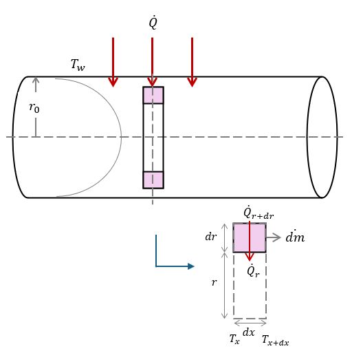
The second case is thermally fully developed flow. In this region, the velocity profile no longer changes along the flow direction. In addition, the dimensionless temperature difference profile no longer varies with the axial distance. Therefore, (Eq 4.4) is satisfied. As in plug flow, heat transfer is dominated by conduction rather than convection. However, unlike plug flow, the velocity varies with radial distance. By expanding (Eq 4.4), we obtatin (Eq 4.5).
(Figure 4.2)
\( {\small\displaystyle\begin{gather} \frac{\partial}{\partial x} \left(\frac{T_w\,-\,T(x,r)}{T_w\,-\,\bar{T}(x)}\right) \quad=\quad 0 \tag{Eq 4.4} \\[15pt] \frac{\partial T}{\partial x} \quad=\quad \frac{\partial T_w}{\partial x} \,-\, \frac{T_w\,-\,T}{T_w\,-\,\bar{T}}\frac{\partial T_w}{\partial x} \,+\, \frac{T_w\,-\,T}{T_w\,-\,\bar{T}}\frac{\partial \bar{T}}{\partial x} \tag{Eq 4.5} \end{gather} } \)
Based on (Figure 4.2), we derive the energy balance equation for a differential element.
\( {\small\displaystyle\begin{align} \dot{Q}_r\,-\,\dot{Q}_{r+dr} \quad&=\quad d\dot{m}C_p\left(T_{x+dx}\,-\,T_x\right) \tag{Eq 4.6} \\[15pt] \dot{Q}_r\,-\,\left(\dot{Q}_r\,+\,\frac{\partial \dot{Q}}{\partial r}\,\cdot\,dr\right) \quad&=\quad d\dot{m}C_p \left[\left(T_x\,+\,\frac{\partial T}{\partial x}\,\cdot\,dx\right)\,-\,T_x\right] \\[15pt] -\frac{\partial \dot{Q}}{\partial r}\,\cdot\,dr \quad&=\quad d\dot{m}C_p\frac{\partial T}{\partial x}\,\cdot\,dx \tag{Eq 4.7} \end{align} } \)
The heat transfer rate (\({\small\displaystyle \dot{Q}_r}\)) can be expressed using definition of heat conduction introduced in Episode 01. The mass flow rate (\({\small\displaystyle \dot{m}}\)) can be written as the product of density (\({\small\displaystyle \rho}\)), velocity (\({\small\displaystyle v}\)) and area (\({\small\displaystyle A}\)). Using these relations, (Eq 4.7) can be rewritten as (Eq 4.8). By replacing the local velocity \({\small\displaystyle v}\) in (Eq 4.8) with the mean velocity \({\small\displaystyle \bar{v}}\) under fuuly developed flow conditions, we obtain (Eq 4.9). (The relationship between the local and mean velocity in fully developed flow will be discussed in detail in another episode.)
\( {\small\displaystyle\begin{align} \partial\dot{Q}_r \,=\, -2\pi rkdx\frac{\partial T}{\partial r} \quad &\& \quad d\dot{m} \,=\,2\pi r\rho v dr \\[15pt] k\frac{1}{\partial r} \left(r\frac{\partial T}{\partial r}\right) \quad&=\quad \rho vr C_p\left(\frac{\partial T}{\partial x}\right) \tag{Eq 4.8} \\[15pt] \frac{1}{\partial r}\left(r\frac{\partial T}{\partial r}\right) \quad&=\quad \frac{2\bar{v}}{\alpha}\frac{\partial T}{\partial x}\left[1\,-\,\left(\frac{r}{r_0}\right)^2\right]r \tag{Eq 4.9} \\[10pt] &\text{where } \,v(r) \,=\, 2\bar{v} \left[1\,-\,\left(\frac{r}{r_0}\right)^2\right] \end{align} } \)
Constant heat flux
Then, what happens if constant heat flux is imposed at the wall under fully developed flow conditions? According to (Eq 1.2), the wall heat flux is
\( {\small\displaystyle\begin{align} \frac{\dot{Q}}{A} \,=\, h(T_w\,-\,\bar{T}) \,=\, \text{constant} \tag*{} \end{align} } \)
Substituting the above expression for \({\small\displaystyle T_w\,-\,\bar{T}}\) into (Eq 4.4) and assuming that \({\small\displaystyle h}\) is constant yields (Eq 4.10). Using this result in (Eq 4.5) gives (Eq 4.11). Therefore, under the constant heat flux condition, (Eq 4.12) is satisfied. Integrating (Eq 4.12) with respect to \({\small\displaystyle r}\) gives an expression for the local temperature \({\small\displaystyle T}\).
\( {\small\displaystyle\begin{align} \frac{\partial T_w}{\partial x} \quad&=\quad \frac{\partial T}{\partial x} \tag{Eq 4.10} \\[15pt] \frac{\partial T}{\partial x} \quad&=\quad \frac{\partial \bar{T}}{\partial x} \tag{Eq 4.11} \\[15pt] \frac{1}{\partial r}\left(r\frac{\partial T}{\partial r}\right) \quad&=\quad \frac{2\bar{v}}{\alpha} \frac{\partial \bar{T}}{\partial x}\left[1\,-\,\left(\frac{r}{r_0}\right)^2\right]r \tag{Eq 4.12} \\[15pt] T(x,r) \quad&=\quad \frac{2\bar{v}}{\alpha}\frac{\partial \bar{T}}{\partial x}\left(\frac{r^2}{4}\,-\,\frac{1}{16r_0^2}\right)\,+\,C_1\ln r\,+\,C_2 \tag{Eq 4.13} \end{align} } \)
Since the following conditions must be satisfied, the local temperature \({\small\displaystyle T(x,r)}\) is a given by:
\( {\small\displaystyle\begin{gather} r\,=\,0 \quad\longrightarrow\quad C_1\,=\,0 \\[10pt] T(x,r_0)\,=\,T_s \quad\longrightarrow\quad C_2\,=\, T_w\,-\,\frac{2\bar{v}}{\alpha}\frac{\partial \bar{T}}{\partial x}\cdot\frac{3r_0^2}{16} \tag*{} \\[15pt] T(x,r) \quad=\quad T_w\,+\, \frac{2\bar{v}}{\alpha}\frac{\partial T_m}{\partial x}\left(\frac{r^2}{4}\,-\,\frac{r^4}{16r_0^2}\,-\,\frac{3r_0^2}{16}\right) \tag{Eq 4.14} \end{gather} } \)
Now, let’s calculate the mean temperature using (Eq 4.2).
\( {\small\displaystyle\begin{align} \bar{T} \quad&=\quad \frac{2}{\bar{v}r_0^2} \int_0^{r_0}\,vTr\,dr \\[15pt] &=\quad \frac{4}{r_0^2} \int_0^{r_0}\,\left(r\,-\,\frac{r^3}{r_0^2}\right)\left[T_w\,+\, \frac{2\bar{v}}{\alpha}\frac{\partial\bar{T}}{\partial x}\left(\frac{r^2}{4}\,-\,\frac{r^4}{16r_0^2}\,-\,\frac{3r_0^2}{16}\right)\right]\,dr \\[15pt] &=\quad T_w\,-\,\frac{11}{48}\frac{\bar{v}r_0^2}{\alpha}\frac{\partial \bar{T}}{\partial x} \tag{Eq 4.15} \end{align} } \)
In (Eq 4.15), the term \({\small\displaystyle \partial\bar{T}/\partial x}\) can be expressed from an energy balance. By going through the following steps, we can obtain the theoretical Nusselt number.
\( {\small\displaystyle\begin{align} d\dot{Q} \,=\, \dot{m}C_pd\bar{T} \,=\, \dot{Q}_A\pi Ddx \quad&\longrightarrow\quad \frac{d\bar{T}}{dx} \,=\, \frac{\dot{Q}_AD}{\rho \bar{v}r_0^2C_p} \,=\, \frac{\alpha \dot{Q}_AD}{\bar{v}r_0^2k} \\[10pt] T_w\,-\,\bar{T} \quad&=\quad \frac{11}{48}\frac{\dot{Q}_AD}{k}, \quad \text{where }\dot{Q}_A\,=\,h\left(T_w\,-\,\bar{T}\right) \tag{Eq 4.16} \\[15pt] \text{Nu} \quad&\approx\quad 4.36 \tag{Ea 4.17} \end{align} } \)
Constant wall temperature
We now consider the case of a constant wall temperature. Under this condition, (Eq 4.5) can be rearranged to give (Eq 4.18).
\( {\small\displaystyle\begin{align} \frac{\partial T}{\partial x} \quad&=\quad \frac{T_w\,-\,T}{T_w\,-\,\bar{T}} \frac{\partial \bar{T}}{\partial x} \tag{Eq 4.18} \\[10pt] \text{Then }\qquad\qquad& \\[10pt] \frac{1}{\partial r} \left(r\frac{\partial T}{\partial r}\right) \quad&=\quad \frac{2\bar{v}}{\alpha} \frac{T_w\,-\,T}{T_w\,-\,\bar{T}} \left[1\,-\,\left(\frac{r}{r_0}\right)^2\right]r \frac{\partial \bar{T}}{\partial x} \tag{Eq 4.19} \end{align} } \)
For mathematical convenience, the following dimensionless variables are defined:
\( {\small\displaystyle\begin{align} \frac{T_w\,-\,T}{T_w\,-\,\bar{T}} \,=\,\theta, \quad \frac{r}{r_0}\,=\,\eta, \quad \frac{\alpha x}{2\bar{v}r_0^2} \,=\,\epsilon \tag*{} \end{align} } \)
Using the newly defined variables, we obtain the following relations.
\( {\small\displaystyle\begin{align} \frac{\partial T}{\partial r} \,=\, -(T_w\,-\,\bar{T})\frac{\partial\theta}{\partial r}, \qquad \frac{\partial^2T}{\partial r^2} \,=\, -(T_w\,-\,\bar{T})\frac{\partial^2\theta}{\partial r^2}, \qquad \partial r \,=\, r_0\partial\eta \tag*{} \end{align} } \)
\( {\small\displaystyle\begin{align} \frac{2\bar{v}}{\alpha}\frac{r_0^2}{T_w\,-\,\bar{T}} \frac{\partial \bar{T}}{\partial x}\left[1\,-\,\eta^2\right]\eta\theta \quad=\quad -\frac{\partial}{\partial\eta}\left(\eta\frac{\partial\theta}{\partial\eta}\right) \tag{Eq 4.20} \end{align} } \)
Note that \({\small\displaystyle \frac{1}{T_w\,-\,\bar{T}}\frac{\partial\bar{T}}{\partial x}}\) is a constant. So why is it constant? To understand this, let’s consider the energy balance at the wall, noting that the change in fluid enthalpy is equal to the heat transfer by conduction.
\( {\small\displaystyle\begin{gather} \dot{m}C_pd\bar{T} \quad=\quad -kdA\left.\frac{\partial T}{\partial r}\right|_{r=r_0} \\[10pt] \frac{d\bar{T}}{dx} \,=\, \frac{-2k}{\rho\bar{v}r_oC_p}\frac{\partial T}{\partial r} \quad\longrightarrow\quad \frac{1}{T_w\,-\,\bar{T}}\frac{d\bar{T}}{dx} \,=\, \frac{2}{\rho\bar{v}r_0C_p}\left.\frac{\partial\theta}{\partial r}\right|_{r=r_0} \tag*{} \end{gather} } \)
In thermally fully developed flow, (Eq 4.5) is satisfied. Therefore, in \({\small\displaystyle \theta(r,x)}\), the x-dependent term acts only as a scaling factor, and the distribution is essentially a function of \({\small\displaystyle r}\). In other words, the value of \({\small\displaystyle \theta'(r_0)}\) remains constant, so we can write the relation as (Eq 4.21)
\( {\small\displaystyle\begin{gather} \frac{2\bar{v}}{\alpha}\frac{r_0^2}{T_w\,-\,\bar{T}}\frac{\partial\bar{T}}{\partial x} \,=\, \lambda^2 \qquad\text{or}\qquad \frac{1}{T_w\,-\,\bar{T}}\frac{\partial\bar{T}}{\partial\epsilon} \,=\, \lambda^2 \tag{Eq 4.21} \end{gather} } \)
Now, let’s solve the differential equation by integrating (Eq 4.21).
\( {\small\displaystyle\begin{gather} \int_{\bar{T}_i}^{\bar{T}}\,\frac{1}{T_w\,-\,\bar{T}}\,d\bar{T} \,=\, \int_0^{\epsilon}\lambda^2\,d\epsilon \quad\longrightarrow\quad \frac{T_w\,-\,\bar{T}}{T_w\,-\,\bar{T}_i} \,=\, \exp\left(-\lambda^2\epsilon\right) \\[15pt] \theta_i \quad=\quad \theta\exp\left(-\lambda^2\epsilon\right) \tag{Eq 4.22} \end{gather} } \)
We can simplify (Eq 4.2) using (Eq 4.21). The corresponding initial and boundary conditions are given as follows.
\( {\small\displaystyle\begin{align} \frac{\partial}{\partial\eta}\left(\eta\frac{\partial\theta}{\partial\eta}\right)\,&+\,\lambda^2\left(1\,-\,\eta^2\right)\eta\theta \quad=\quad 0 \tag{Eq 4.23} \\[15pt] \theta(1,\epsilon) \quad&=\quad 0\quad \text{for all } \epsilon \\[10pt] \theta'(0) \quad&=\quad 0 \\[10pt] \theta(r,0) \quad&=\quad 1 \end{align} } \)
Let \({\small\displaystyle \theta}\) be expressed as a power series solution. Substituting (Eq 4.24) into (Eq 4.23) and simplifying yields a recurrence relation for the coefficients \({\small\displaystyle a_n}\). For normalization, we set \({\small\displaystyle a_0\,=\,1}\). Furthermore, by taking the order in (Eq 4.24) as \({\small\displaystyle 2n}\), the solution satisfies symmetry about the centerline.
\( {\small\displaystyle\begin{gather} \theta(\eta) \quad=\quad \sum_{n=1}^{\infty}\, A_n\phi_n(\eta) \qquad \text{where } \,\phi_n(\eta) \,=\, \sum_{n=0}^{\infty}\, a_n(\lambda)\eta^{2n} \tag{Eq 4.24} \\[15pt] \phi'_n(\eta) \,=\, \sum_{n=1}^{\infty}\, 2na_n(\lambda)\eta^{2n-1},\qquad \phi''_n(\eta) \,=\, \sum_{n=1}^{\infty}\, 2n(2n-1)a_n(\lambda)\eta^{2n-2} \\[15pt] \eta^2\phi''\,+\,\eta\phi'\,+\,\lambda^2\phi\left(1\,-\,\eta^2\right)\eta^2 \quad=\quad 0 \tag{Eq 4.25} \\[15pt] \left(\lambda^2a_0\,+\,4a_1\right)\eta^2\,+\,\sum_{n=1}^{\infty}\,\left(4n^2a_n\,+\,\lambda^2a_{n-1}\,-\,\lambda^2a_{n-2}\right)\eta^{2n} \quad=\quad 0 \tag{Eq 4.26} \\[15pt] a_1\,=\, -\frac{\lambda^2}{4},\quad a_n\,(n\ge 2)\,=\, \frac{\lambda^2\left(a_{n-2}\,-\,a_{n-1}\right)}{4n^2} \tag{Eq 4.27} \end{gather} } \)
The eigenvalues \({\small\displaystyle \lambda}\) are the values that satisfy \({\small\displaystyle \theta\,=\,1}\) at \({\small\displaystyle \eta\,=\,1}\). (i.e, at the wall)
\( {\small\displaystyle\begin{align} \sum_{n=0}^{\infty} \,a_n(\lambda) \quad=\quad 0 \tag{Eq 4.28} \end{align} } \)
Now, let’s determine the coefficient \({\small\displaystyle A_n}\) in (Eq 4.24) using the initial condition. Since \({\small\displaystyle \theta}\) satisfies a Sturm-Liouville equation, it can be expressed in the following form, where the weight function \({\small\displaystyle w(\eta)\,=\,\eta\left(1\,-\,\eta^2\right)}\).
\( {\small\displaystyle\begin{align} 1 \quad&=\quad \sum_{n=1}^{\infty}\, A_n\phi_n(\eta) \\[10pt] A_n \quad&=\quad \frac{(1,\phi_n)}{||\phi_n||^2} \quad=\quad \frac{\int_0^1\,w(\eta)\phi_n(\eta)\,d\eta}{\int_0^1\,w(\eta)\phi_n^2(\eta)\,d\eta} \\[10pt] &=\quad \frac{\int_0^1\,\eta\left(1\,-\,\eta^2\right)\phi_n(\eta)\,d\eta} {\int_0^1\,\eta\left(1\,-\,\eta^2\right)\phi_n^2(\eta)\,d\eta} \tag{Eq 4.29} \end{align} } \)
As discussed earlier, the \({\small\displaystyle\bar{\theta}_i}\) can be obtained using (Eq 4.2). Defining the coefficient of the \({\small\displaystyle\bar{\theta}_i}\) as \({\small\displaystyle G_n}\) , and substituting (Eq 4.29), we can rewrite the expression as follows.
\( {\small\displaystyle\begin{align} \bar{\theta}_i \quad&=\quad \frac{2}{\bar{v}r_0^2}\int_0^{\infty}\,u\theta_ir\,dr \quad=\quad 4\int_0^{\infty}\,\eta\left(1\,-\,\eta^2\right)\theta_i\,d\eta \\[10pt] &=\quad \sum_{n=0}^{\infty}\, G_n\exp(-\lambda_n^2\epsilon) \tag{Eq 4.30} \\[10pt] &\qquad \text{where } \, G_n\,=\, 4\sum_{n=0}^{\infty} \, \frac {\left\{\int_0^1\, \eta\left(1\,-\,\eta^2\right)\phi_n(\eta) \,d\eta\right\}^2} {\int_0^1\,\eta\left(1\,-\,\eta^2\right)\phi^2_n(\eta)\,d\eta} \end{align} } \)
The denominators of coefficients \({\small\displaystyle A_n}\) and \({\small\displaystyle G_n}\) can be evaluated numerically using Simpson’ rule. The numerical values are listed in (Table 4.2). (There are may be slight differences compared to other references, but these are due to differences in accuracy and have a negligible effect.) From (Table 4.2), we observe that \({\small\displaystyle G_n}\) decreases rapidly as n increases.Therefore, in evaluating the \({\small\displaystyle \bar{\theta}_i}\) , the contribution of higher-order terms can be considered negligible. Based on this approximation, the theoretical Nusselt number can be obtained using only the first term.
\( {\small\displaystyle\begin{align} \bar{\theta}_i \quad&=\quad G_1\exp\left(\frac{-\alpha\lambda_1^2}{2\bar{v}r_0^2}x\right) \tag*{} \end{align} } \)
| n | \({\small\displaystyle\lambda_n}\) | \({\small\displaystyle A_n}\) | \({\small\displaystyle G_n}\) |
|---|---|---|---|
| 1 | 2.704 | 1.476 | 0.81905 |
| 2 | 6.679 | -0.806 | 0.09753 |
| 3 | 10.673 | 0.589 | 0.0325 |
| 4 | 14.671 | -0.476 | 0.01544 |
| 5 | 18.670 | 0.405 | 0.00879 |
By differentiating \({\small\displaystyle \bar{\theta}_i}\) with respect to \({\small\displaystyle x}\) and substituting for \({\small\displaystyle d\bar{T}/dx}\), as in the constant heat flux case, the following result is obtained.
\( {\small\displaystyle\begin{gather} \frac{d\bar{\theta}_i}{dx} \quad=\quad -\frac{1}{T_w\,-\,T_i}\frac{d\bar{T}}{dx} \quad=\quad -\frac{\alpha\lambda^2_1G_1}{2\bar{v}r_0^2}\exp\left(\frac{-\alpha\lambda_1^2}{2\bar{v}r_0^2}x\right) \\[10pt] \frac{1}{T_w\,-\,T_i} \frac{\dot{q}D}{k} \,=\, \frac{G_1\lambda^2_1}{2}\exp\left(\frac{-\alpha\lambda_1^2}{2\bar{v}r_0^2}x\right) \quad\longrightarrow\quad \frac{hD}{k}\bar{\theta}_i \,=\, \frac{\lambda^2_1G_1}{2}\exp\left(\frac{-\alpha\lambda_1^2}{2\bar{v}r_0^2}x\right) \\[15pt] \text{Nu} \quad\approx\quad 3.66 \tag{Eq 4.31} \end{gather} } \)
The theoretical Nusselt number obtained so far corresponds to the case where the Graetz number approaches zero. It means that the flow is sufficiently far from the inlet and thermally fully developed conditions have been established. So, how does the Nusselt number change in the entrance region? Near the inlet, the flow can be hydrodynamically fully developed while still being thermally developing. This behavior is typically observed for fluids with large Prandtl numbers.

(Figure 4.3)
First, for a constant wall temperature, the Nusselt number can be expressed as a function of the Graetz number, as follows.
\( {\small\displaystyle\begin{align} \dot{Q} \quad&=\quad hA\Delta T_L \\[10pt] &=\quad h(\pi DL)\frac{T_i\,-\,\bar{T}_0}{\ln\left[(T_w\,-\,\bar{T}_0)/(T_w\,-\,T_i)\right]} \\[10pt] &=\quad \dot{m}C_p\left(T_0\,-\,\bar{T}_i\right) \\[10pt] h \quad&=\quad \frac{\dot{m}C_p}{\pi DL}\ln\left(\frac{T_w\,-\,T_i}{T_w\,-\,\bar{T}_0}\right) \\[15pt] \bar{\text{Nu}} \quad&=\quad \frac{\text{Gz}}{\pi} \ln\left(\frac{T_w\,-\,T_i}{T_w\,-\,\bar{T}_0}\right) \tag{Eq 4.32} \end{align} } \)
For the constant heat flux condition, the Nusselt number can be obtained not only through mathematical analysis but also from analytical correlations. A representative example is (Eq 4.33), proposed by Shah and London.
\( {\small\displaystyle\begin{align} \bar{\text{Nu}} \quad=\quad \begin{cases} 1.953 x^{*(-1/3)}& x^*\,\le\,0.03\\[10pt] 4.364\,+\,0.0722/x^*& x^*\,>\,0.03 \end{cases} \tag{Eq 4.33} \\[10pt] \text{where }\quad x^* \,=\, 1/\text{Gz} \end{align} } \)
(Figure 4.3) presents (Eq 4.32) and (Eq 4.33) graphically. For both correlations, the Nusselt number approaches the theoretical value obtained earlier as the Graetz number decreases toward zero.
Viscosity is also an important factor in heat transfer. For fluids with large viscosity variations due to temperature changes, the heat transfer behavior near the wall differs from that near the flow center. Therefore, the influence of viscosity variation should also be considered. To account for this effect, a correction factor is introduced.
\( {\small\displaystyle\begin{align} \phi_v \quad=\quad \left(\frac{\mu}{\mu_w}\right)^{0.14} \tag{Eq 4.34} \end{align} } \)
Applying this to (Eq 4.32) yields the following expression.
\( {\small\displaystyle\begin{align} \bar{\text{Nu}} \quad=\quad \frac{\text{Gz}}{\pi}\ln\left(\frac{1}{\bar{\theta_i}}\right)\phi_v \tag{Eq 4.35} \end{align} } \)
Nomenclature
\({\small\displaystyle A}\) : area
\({\small\displaystyle \text{Bi}}\) : Biot number
\({\small\displaystyle C_p}\) : heat capacity
\({\small\displaystyle D}\) : diameter
\({\small\displaystyle \text{Fo}}\) : Fourier number
\({\small\displaystyle \text{Gz}}\) : Graetz number
\({\small\displaystyle h}\) : heat transfer coefficient
\({\small\displaystyle k}\) : thermal conductivity
\({\small\displaystyle L}\) : length
\({\small\displaystyle \dot{m}}\) : mass flowrate
\({\small\displaystyle \text{Nu}}\) : Nusselt number
\({\small\displaystyle \bar{\text{Nu}}}\) : mean Nusselt number
\({\small\displaystyle \text{Pe}}\) : Peclect number
\({\small\displaystyle \text{Pr}}\) : Prandtl number
\({\small\displaystyle \dot{Q}}\) : the rate of heat
\({\small\displaystyle \dot{Q}_A}\) : heat flux
\({\small\displaystyle \text{Ra}}\) : Rayleigh number
\({\small\displaystyle \text{Re}}\) : Reynolds number
\({\small\displaystyle r}\) : radius
\({\small\displaystyle r_o}\) : radius to the wall
\({\small\displaystyle \text{St}}\) : Stanton number
\({\small\displaystyle T}\) : temperature
\({\small\displaystyle T_i}\) : inlet temperature
\({\small\displaystyle T_o}\) : outlet temperature
\({\small\displaystyle T_w}\) : outlet temperature
\({\small\displaystyle \bar{T}}\) : mean temperature
\({\small\displaystyle v}\) : velocity
\({\small\displaystyle \bar{v}}\) : mean velocity
\({\small\displaystyle x}\) : x-axis variable
\({\small\displaystyle \alpha}\) : thermal diffusivity
\({\small\displaystyle \rho}\) : density
\({\small\displaystyle \theta,\,\eta,\,\epsilon}\) : dimensionless variables
\({\small\displaystyle \phi_v}\) : viscosity correction factor
\({\small\displaystyle \lambda}\) : eigenvalues