Episode 02. Conduction - Steady State
Summary
This episode covers conduction-one of the three modes of heat transfer. We start by examining thermal conductivity and derive the general conduction equation. Finally, we discuss how to calculate conduction under steady-state conditions for specific scenarios.
1. Introduction
Before delving into conduction, we review thermal conductivity, as introduced in a previous episode. Although (Eq 1.1) treats \({\small\displaystyle k}\) as a constant, it is not independent of temperature in reality. Within a narrow temperature range, \({\small\displaystyle k}\) can be reasonably assumed to be constant. However, over a broader range, it may increase or decrease with temperature. In general, thermal conductivity varies linearly with temperature. But in this episode, we assume it to remain constant regardless of the temperature range.
\( {\small\displaystyle\begin{align} k \quad=\quad k_0(1\,+\,\gamma T) \tag{Eq 2.1} \end{align} } \)
The form of Fourier’s Law, which describes heat transfer across an infinitesimal area, is (Eq 2.2). \({\small\displaystyle \dot{Q}}\) in (Eq 2.2) can be replaced by a change of heat quantity with respect to time.
\( {\small\displaystyle\begin{align} d\dot{Q} \quad&=\quad -kdA\frac{dT}{dx} \tag{Eq 2.2} \\[15pt] \frac{dQ}{dt} \quad&=\quad -kdA\frac{dT}{dx} \tag{Eq 2.3} \end{align} } \)
2. Derivation of general equation for conduction
(Figure 2.1)
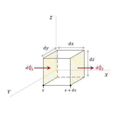
To derive the general equation for heat transfer by conduction, let us consider an object of volume \({\small\displaystyle dxdydz}\), as shown in (Figure 2.1). Assume that heat flows in the x-direction. \({\small\displaystyle d\dot{Q}_1}\) refers to the rate of heat entering the object, and \({\small\displaystyle d\dot{Q}_2}\) is the rate of heat leaving it. Using (Eq 2.3), \({\small\displaystyle d\dot{Q}_1}\) and \({\small\displaystyle d\dot{Q}_2}\) can be expressed as follows:
\( {\small\displaystyle\begin{align} \frac{dQ_1}{dt} \quad&=\quad -kdydz\left(\frac{dT}{dx}\right) \tag{Eq 2.4} \\[15pt] \frac{dQ_2}{dt} \quad&=\quad -kdydz\left(\frac{dT}{dx}\,+\,\frac{\partial^2 T}{\partial x^2}dx\right) \tag{Eq 2.5} \end{align} } \)
Thus, the accumulation in heat within the object is given by the following expression.
\( {\small\displaystyle\begin{align} d\dot{Q}' \quad&=\quad d\dot{Q}_1\,-\,d\dot{Q}_2 \\[15pt] \frac{dQ'}{dt} \quad&=\quad kdxdydz\frac{\partial^2 T}{\partial x^2} \tag{Eq 2.6} \end{align} } \)
The left-hand side of (Eq 2.6) can be rewritten using properties, including heat capacity and density.
\( {\small\displaystyle\begin{align} \frac{dQ'}{dt} \quad&=\quad \rho C_pV\frac{dT}{dt} \tag{Eq 2.7} \\[15pt] &=\quad \rho C_pdxdydz\frac{dT}{dt} \end{align} } \)
Therfore,
\( {\small\displaystyle\begin{align} \frac{dT}{dt} \quad=\quad \frac{k}{\rho C_p}\frac{\partial^2 T}{\partial x^2} \quad=\quad \alpha\frac{\partial^2 T}{\partial x^2} \tag{Eq 2.8} \end{align} } \)
The parameter \({\small\displaystyle \alpha}\) in (Eq 2.8) represents thermal diffusivity. For isotropic materials, the equation can be generalized to three dimensions as follows.
\( {\small\displaystyle\begin{align} \frac{dT}{dt} \quad=\quad \frac{k}{\rho C_p}\left(\frac{\partial^2 T}{\partial x^2} \,+\, \frac{\partial^2T}{\partial y^2} \,+\, \frac{\partial^2T}{\partial z^2} \right) \tag{Eq 2.9} \end{align} } \)
3. Conduction under steady state
Assuming that \({\small\displaystyle Q}\) is constant with respect to time, i.e., under steady-state conditions, we obtain:
\( {\small\displaystyle\begin{align} \frac{dQ'}{dt} \,=\, 0,\qquad \frac{\partial^2 T}{\partial x^2} \,=\, 0 \tag*{} \end{align} } \)
Therefore, (Eq 2.2) is satisfied. For isotropic materials, the equation can be generalized to various coordinate systems.
\( {\small\displaystyle\begin{align} \frac{d\dot{Q}}{dA} \quad&=\quad -k\left(\frac{\partial T}{\partial x}\,+\,\frac{\partial T}{\partial y}\,+\,\frac{\partial T}{\partial z}\right) \tag{Eq 2.10} \\[15pt] \frac{d\dot{Q}}{dA} \quad&=\quad -k\left(\frac{\partial T}{\partial r}\,+\,\frac{1}{r}\frac{\partial T}{\partial\theta}\,+\,\frac{\partial T}{\partial z}\right)\qquad \text{(In cylindrical coordinates)} \tag{Eq 2.11} \\[15pt] \frac{d\dot{Q}}{dA} \quad&=\quad -k\left(\frac{\partial T}{\partial r}\,+\,\frac{1}{r}\frac{\partial T}{\partial\theta}\,+\,\frac{1}{r\sin\theta}\frac{\partial T}{\partial\phi}\right)\qquad \text{(In spherical coordinates)} \tag{Eq 2.12} \end{align} } \)
If the temperature profile is linear and the heat transfer area is constant, (Eq 2.2) can be simplified as follows. Here, \({\small\displaystyle R}\) denotes the thermal resistance, defined as the thickness of the material divided by its thermal conductivity.
\( {\small\displaystyle\begin{align} \dot{Q} \quad=\quad -kA\frac{\Delta T}{\Delta x} \quad=\quad -A\frac{\Delta T}{R} \tag{Eq 2.13} \end{align} } \)
(Figure 2.2)
Thermal resistance in series
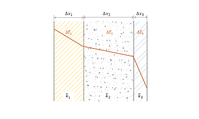
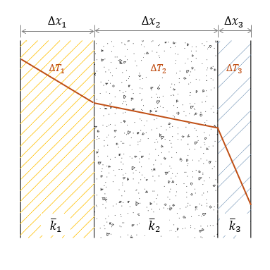
Then, what happens when different thermal resistances-i.e., multiple solids-are arranged in series? Let us consider a case where objects with different thermal conductivities are connected in series, as shown in (Figure 2.2). If there is no temperature drop at the interfaces, the total temperature difference can be expressed as follows.
\( {\small\displaystyle\begin{align} \Delta T_t \quad=\quad \Delta T_1 \,+\, \Delta T_2 \,+\, \Delta T_3 \tag*{} \end{align} } \)
Under steady-state conditions, the rate of heat is constant across all segments. Therefore, assuming the rate of heat is denoted by \({\small\displaystyle \dot{Q}}\), we can express the temperature gradient in each section using (Eq 2.13) accordingly.
\( {\small\displaystyle\begin{align} \Delta T_1 \,=\, -\frac{\dot{Q}}{\bar{k}_1A}\Delta x_1, \qquad \Delta T_2 \,=\, -\frac{\dot{Q}}{\bar{k}_2A}\Delta x_2, \qquad \Delta T_3 \,=\, -\frac{\dot{Q}}{\bar{k}_3A}\Delta x_3 \tag*{} \end{align} } \)
Since the sum of the individual temperature differences equals the total temperature difference, this relationship is given by the following expression.
\( {\small\displaystyle\begin{align} \Delta T_t \quad&=\quad -\left(\frac{\dot{Q}}{\bar{k}_1A}\Delta x_1, \,+\, \frac{\dot{Q}}{\bar{k}_2A}\Delta x_2 \,+\, \frac{\dot{Q}}{\bar{k}_3A}\Delta x_3 \right) \\[15pt] \frac{\dot{Q}}{A} \quad&=\quad -\frac{\Delta T_t}{R_1\,+\,R_2\,+\,R_3} \tag{Eq 2.14} \end{align} } \)
Based on (Eq 2.13) and (Eq 2.14), we can conclude that the total thermal resistance is equivalent to the sum of the individual thermal resistances.
\( {\small\displaystyle\begin{align} R_t \quad=\quad R_1\,+\,R_2\,+\,R_3 \tag{Eq 2.15} \end{align} } \)

(Figure 2.3)
Conduction in cylindrical coordinates
Now, let’s examine steady-state conduction in a cylindrical geometry (such as a pipe). The heat flux through the pipe can be derived using (Eq 2.11). Assuming heat is transferred only by conduction in the radial direction, it can be expressed as (Eq 2.16).
\( {\small\displaystyle\begin{align} \frac{\dot{Q}}{2\pi rL} \quad&=\quad -k\frac{dT}{dr} \tag{Eq 2.16} \\[15pt] \int_{r_i}^{r_o}\,\frac{dr}{r} \quad&=\quad -\int_{T_i}^{T_o}\,\frac{2\pi kL}{\dot{Q}}\,dT \end{align} } \)
By integrating from \({\small\displaystyle r_i}\) to \({\small\displaystyle r_o}\) and rearranging the equation, we obtain (Eq 2.17). \({\small\displaystyle A_L}\) denotes the logarithmic mean area, and \({\small\displaystyle r_L}\) represents the logarithmic mean radius.
\( {\small\displaystyle\begin{align} \dot{Q} \quad&=\quad \frac{2\pi kL(T_i\,-\,T_o)}{\ln r_o\,-\,\ln r_i} \quad=\quad \frac{k\bar{A}_L(T_i\,-\,T_o)}{r_o\,-\,r_i} \tag{Eq 2.17} \\[15pt] \bar{A}_L \quad&=\quad \frac{2\pi L(r_o\,-\,r_i)}{\ln r_o\,-\,\ln r_i} \quad=\quad 2\pi\bar{r}_LL \tag{Eq 2.18} \\[15pt] \bar{r}_L \quad&=\quad \frac{r_o\,-\,r_i}{\ln r_o\,-\,\ln r_i} \tag{Eq 2.19} \end{align} } \)
Nomenclature
\({\small\displaystyle A}\) : area
\({\small\displaystyle \bar{A}}\) : logarithmic mean area
\({\small\displaystyle C_p}\) : heat capacity
\({\small\displaystyle k}\) : thermal conductivity
\({\small\displaystyle \bar{k}}\) : average thermal conductivity
\({\small\displaystyle L}\) : length
\({\small\displaystyle Q}\) : the quantity of heat
\({\small\displaystyle \dot{Q}}\) : rate of heat
\({\small\displaystyle R}\) : thermal resistance
\({\small\displaystyle r}\) : radius
\({\small\displaystyle \bar{r}}\) : logarithmic mean radius
\({\small\displaystyle T}\) : temperature
\({\small\displaystyle t}\) : time
\({\small\displaystyle \Delta x}\) : thickness
\({\small\displaystyle \alpha}\) : thermal diffusivity
\({\small\displaystyle \gamma}\) : coefficient
\({\small\displaystyle \rho}\) : density