Episode 05. Bimetallic Thermometer
Summary
The bimatallic thermometer is a widely used type of thermometer that operates based on the difference in thermal expansion between two metals. In this episode we describe how bimetal strips respond to temperature changes depending on their configuration and introduce the features of bimetallic thermometers.
1. Introduction
A bimetallic thermometer is a device that measures temperature based on the difference in thermal expansion between two metals. When two dissimilar metal strips are bonded together, and one has a higher thermal expansion coefficient than the other, the metal strip bends toward the side with the lower expansion coefficient. This principle is widely applied in field temperature gauges, temperature sensors, and so on. We discuss how various types of bimetallic devices respond to temperature changes.
\( {\small\displaystyle\begin{align} &\text{Coefficient of linear expansion} \\[10pt] &\alpha\Delta T \quad=\quad \frac{\Delta L}{L} \\[15pt] &\text{Young's moduls} \\[10pt] &E \quad=\quad \frac{\sigma}{\epsilon} \\[15pt] &\text{Relationship between bending moment and curvature} \\[10pt] &\frac{1}{R} \quad=\quad \frac{M}{EI} \end{align} } \)
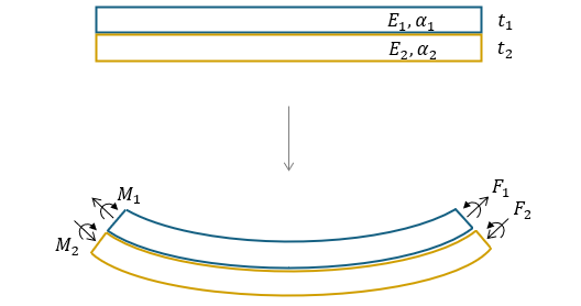
(Figure 5.1)
2. Working principle and configuration of bimetal strips
Consider two different metals bonded together in a strip form, as shown in (Figure 5.1). The metal with the lower expansion coefficient (\({\small\displaystyle\alpha_1}\)) undergoes tensile force (\({\small\displaystyle F_1}\)), while the metal with the higher expansion coefficient (\({\small\displaystyle\alpha_2}\)) undergoes compressive force (\({\small\displaystyle F_2}\)). If we define the bending moments acting on each metal strip as \({\small\displaystyle M_1}\) and \({\small\displaystyle M_2}\), we can derive equations (5.1) to (5.3). Subscript ‘0’ represents the initial state.
\( {\small\displaystyle\begin{align} F \quad&=\quad F_1 \quad=\quad -\,F_2 \tag{Eq 5.1} \\[15pt] \frac{\left(F\,-\,F_0\right)t}{2} \quad&=\quad (M_1\,-\,M_{01}) \,+\, (M_2\,-\,M_{02}) \tag{Eq 5.2} \\[15pt] &=\quad \left(E_1I_1\,+\,E_2I_2\right)\cdot \left(\frac{1}{R}\,-\,\frac{1}{R_0}\right) \tag{Eq 5.3} \end{align} } \)
When deriving the equation for strain (\({\small\displaystyle \epsilon}\)), it is expressed as shown in (Eq 5.4).
\( {\small\displaystyle\begin{align} \alpha_1\left(T\,-\,T_0\right) \,+\, \frac{F_1\,-\,F_0}{E_1t_1} &\,+\, \frac{t_1}{2}\left(\frac{1}{R}\,-\,\frac{1}{R_0}\right) \\ \tag{Eq 5.4} \\ =\quad&\alpha_2\left(T\,-\,T_0\right) \,+\, \frac{F_2\,-\,F_0}{E_2t_2} \,-\, \frac{t_2}{2}\left(\frac{1}{R}\,-\,\frac{1}{R_0}\right) \end{align} } \)
Rearranging (Eq 5.4) with (Eq 5.1) and (Eq 5.3) yields the following expression.
\( {\small\displaystyle\begin{align} \frac{1}{R}\,-\,\frac{1}{R_0} \quad&=\quad \frac{(\alpha_2\,-\,\alpha_1)(T\,-\,T_0)}{\dfrac{t}{2}\,+\,\dfrac{2(E_1I_1\,+\,E_2I_2)}{t}\left(\dfrac{1}{E_1t_1}\,+\,\dfrac{1}{E_2t_2}\right)} \tag*{} \end{align} } \)
Substituting
\( {\small\displaystyle\begin{align} \frac{t_1}{t_2} \,=\,m,\quad \frac{E_1}{E_2} \,=\,n,\quad I_1 \,=\,\frac{t_1^3}{12},\quad \text{and}\quad I_2 \,=\,\frac{t_2^3}{12} \tag*{} \end{align} } \)
results in (Eq 5.5). It is the general equation for the curvature of a bimetallic strip in the absence of external forces.
\( {\small\displaystyle\begin{align} \frac{1}{R}\,-\,\frac{1}{R_0} \quad&=\quad \frac{6(1\,+\,m)^2\left(\alpha_2\,-\alpha_1\right)\left(T\,-\,T_0\right)}{t\left[3\left(1\,+\,m\right)^2\,+\,(1\,+\,mn)\left(m^2\,+\,\dfrac{1}{mn}\right)\right]} \tag{Eq 5.5} \\[10pt] \text{where }\, m\,=\,1,\quad n\,=\,1\quad& \\[10pt] \frac{1}{R}\,-\,\frac{1}{R_0} \quad&=\quad \frac{3(\alpha_2\,-\,\alpha_1)(T\,-\,T_0)}{2t} \\[10pt] \quad&=\quad \frac{k(T\,-\,T_0)}{t},\quad k\,=\,\frac{3}{2}(\alpha_2\,-\,\alpha_1) \tag{Eq 5.6} \end{align} } \)
The \({\small\displaystyle k}\) in (Eq 5.6) is known as flexivity or specific curvature.
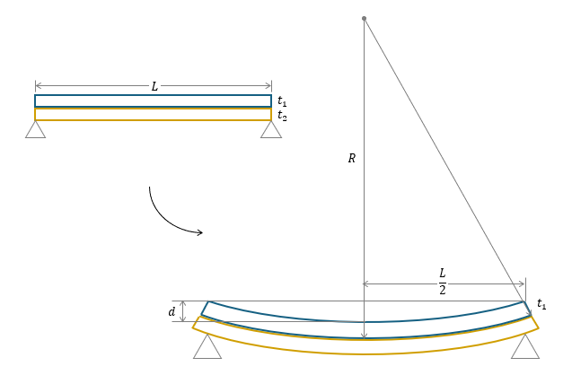
(Figure 5.2)
Bimetallic strip is supported at its end
In the first case, both ends of the strip are supported. In (Figure 5.2), the strip’s length is \({\small\displaystyle L}\), the deflection length is \({\small\displaystyle d}\), and the thicknesses of the two metals are \({\small\displaystyle t_1}\) and \({\small\displaystyle t_2}\). Then, we can establish the following relationship.
\( {\small\displaystyle\begin{gather} \left(R\,-\,d\,-\,t_1\right)^2 \,+\, \left(\frac{L}{2}\right)^2 \quad=\quad \left(R\,-\,t_1\right)^2 \\[10pt] \frac{1}{R} \,=\, \frac{8d}{4d^2\,+\,8dt_1\,+\,L^2} \,\approx\, \frac{8d}{L^2} \tag{Eq 5.7} \end{gather} } \)
Since \({\small\displaystyle L^2}\) is significantly larger than the other terms (\({\small\displaystyle L^2\,\gg\,4d^2,\,8dt}\)), it can be expressed as shown in (Eq 5.7). By substituting this equation into (Eq 5.6), we obtain the following expression:
\( {\small\displaystyle\begin{align} k \quad=\quad \frac{8dt}{(T\,-\,T_0)L^2} \tag{Eq 5.8} \end{align} } \)

(Figure 5.3)
Cantiever strip
The second case consists of a cantilever strip, where one side is fixed, and the other is free to move. As in the first case, we can obtain (Eq 5.9) by deriving and then simplifying the following equation.
\( {\small\displaystyle\begin{gather} \left(R\,-\,d\,+\,t_2\right)^2 \,+\, \left(\frac{L}{2}\right)^2 \quad=\quad \left(R\,+\,t_2\right)^2 \\[10pt] \frac{1}{R} \,=\, \frac{2d}{d^2\,-\,2dt_2\,+\,L^2} \,\approx\, \frac{2d}{L^2} \tag{Eq 5.9} \end{gather} } \)
Using (Eq 5.6) and (Eq 5.9), we can caculate the deflection resulting from temperature changes. Furthermore, by rearranging the equation as shown in (Eq 5.11), we obtain the specific deflection, denoted as ‘\({\small\displaystyle a}\)’. Theoretically, the specific deflection is equal to \({\small\displaystyle k}\).
\( {\small\displaystyle\begin{align} d \quad&=\quad \frac{kL^2\left(T\,-\,T_0\right)}{2t} \tag{Eq 5.10} \\[15pt] a \quad&=\quad \frac{dt}{L^2\left(T\,-\,T_0\right)} \,=\, \frac{k}{2} \tag{Eq 5.11} \end{align} } \)
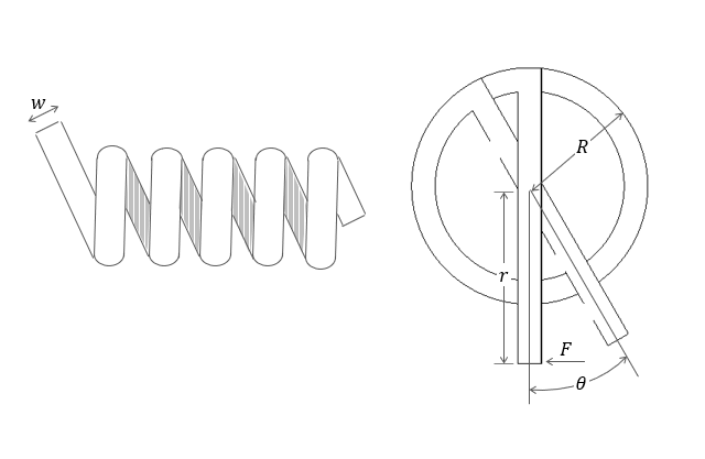
(Figure 5.4)
Spiral and Helical Coil
The spiral and helical coil configuration is commonly found in dial thermometers. A pointer is attached at the end, which moves to indicate the measured temperature in response to temperature changes. Now, let’s analyze the variation in the angular rotation within this configuration.
\( {\small\displaystyle\begin{align} \theta \,=\, \left(\frac{1}{R}\,-\,\frac{1}{R_0}\right)L \,\longrightarrow\, \frac{L}{R} \tag*{} \end{align} } \)
The angular rotation is affected by temperature changes and the mechanical resistance of the pointer.
- Temperature changes
\( {\small\displaystyle\begin{align} \frac{L}{R} \quad&=\quad \frac{kL(T\,-\,T_0)}{t}\cdot \frac{360^{\circ}}{2\pi} \\[10pt] &=\quad \frac{2aL(T\,-\,T_0)}{t}\cdot \frac{360^{\circ}}{2\pi} \tag*{} \end{align} } \)
- Mechanical force
\( {\small\displaystyle\begin{align} \frac{L}{R} \quad&=\quad \frac{ML}{EI}\cdot \frac{360^{\circ}}{2\pi} \\[10pt] &=\quad \frac{12(F\,-\,F_0)rL}{Ewt^3}\cdot\frac{360^{\circ}}{2\pi} \tag*{} \end{align} } \)
Therefore, the angular rotation due to these two factors is expressed as follows.
\( {\small\displaystyle\begin{align} \theta \quad=\quad \left[\frac{2aL(T\,-\,T_0)}{t}\,-\,\frac{12(F\,-\,F_0)rL}{Ewt^3}\right]\cdot\frac{360^{\circ}}{2\pi} \tag{Eq 5.12} \end{align} } \)
3. Features of bimetallic thermometer
In addition to the configurations discussed above, there are other designs available. The appropriate bimetal configuration can be selected and utilized accordingly. For example, a cantilever-type bimetal can be used as a switch that stops the flow of current when a specific temperature is reached. Meanwhile, spiral or helical configurations are commonly used in industrial temperature gauges by attaching a pointer to indicate temperature changes.
A bimetallic thermometer can be used easily without an external power source and measure a wide range of temperatures. It is a relatively inexpensive device, though the cost can increase depending on the types of metals used. However, when selecting this type of thermometer, it is important to ensure that the operating temperature falls within an appropriate range. This is because the deflection of the metal is not linear across all temperature ranges, leading to decreased accuracy when the temperature exceeds a certain limit.
Nomenclature
\({\small\displaystyle a}\) : specific deflection
\({\small\displaystyle d}\) : deflection
\({\small\displaystyle E}\) : Young’s modulus
\({\small\displaystyle F}\) : Force
\({\small\displaystyle I}\) : second moment of area
\({\small\displaystyle k}\) : flexivity or specific curvature
\({\small\displaystyle L}\) : length
\({\small\displaystyle \Delta M}\) : moment
\({\small\displaystyle R}\) : radius
\({\small\displaystyle T}\) : temperature
\({\small\displaystyle t}\) : thickness
\({\small\displaystyle \alpha}\) : coefficient of expansion
\({\small\displaystyle \epsilon}\) : strain
\({\small\displaystyle \theta}\) : angular rotation