
Episode 04. Thermocouple Thermometer
Summary
Thermocouple thermometers are widely used for temperature measurement. This episode covers the principle of thermocouples and various components. We describe various metal combinations, extension lead types, and the different types of junctions.
1. Introduction
Thermocouple thermometers are widely used because they measure a wide range of temperatures and are relatively inexpensive. Thermocouple thermometers use the Seebeck effect to measure temperature.
Seebeck effect
If two different metals form a closed circuit and one junction is at a higher temperature than the other, current flows through the circuit.

(Figure 4.1)
Using the Seebeck coefficient, we can express the change in thermoelectric emf according to the temperature change of each metal. The absolute Seebeck coefficient \({\small\displaystyle S_i}\) is a material property but difficult to measure directly.
\( {\small\displaystyle\begin{align} \Delta E_i \,=\, \int_{T_1}^{T_2}\,S_i(T)\,dT \,=\,E_i(T_2)\,-\,E_i(T_1) \tag{Eq 4.1} \end{align} } \)
As mentioned earlier, a thermocouple forms a junction between two metals. The generated emf in the circuit is:
\( {\small\displaystyle\begin{align} E_{AB}(T_m,\,T_r) \quad=\quad E_A(T_m,\,T_r)\,-\,E_B(T_m,\,T_r) \tag{Eq 4.2} \end{align} } \)
\({\small\displaystyle E_{AB}}\) is relative Seebeck emf, which is the difference between the emfs of metals A and B. \({\small\displaystyle T_m}\) is the temperature at the junction, and \({\small\displaystyle T_r}\) is the reference temperature of both metals. The relative Seebeck coefficient between two metals is:
\( {\small\displaystyle\begin{align} S_{AB}(T_m,\,T_r) \quad=\quad S_A(T_m,\,T_r)\,-\,S_B(T_m,\,T_r) \tag{Eq 4.3} \end{align} } \)
By setting the reference temperature to 0°C, the generated emf due to temperature can be approximated as follows. Constants in (Eq 4.4) vary depending on the metal combinations.
\( {\small\displaystyle\begin{align} E \quad\approx\quad a_1T\,+\,a_2T^2 \tag{Eq 4.4} \end{align} } \)
2. Components of thermocouple
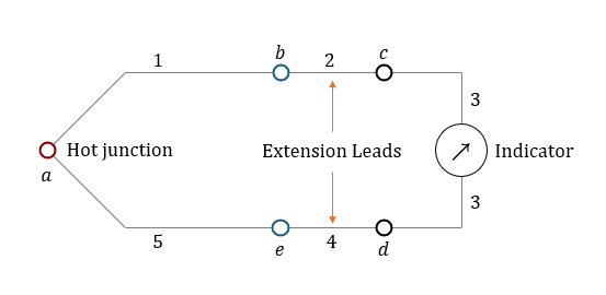
(Figure 4.2) shows the circuit of a thermocouple thermometer. In the figure, two different metal wires form a junction, and extension leads connect each metal wire to the output device. The temperatures at junctions b and e are the same, and the temperatures at junctions c and d are the same.The emf at each junction and the net emf measured by the indicator have the following relationship:
\( {\small\displaystyle\begin{align} E_m \quad=\quad E_a\,+\,E_b\,+\,E_c\,+\,E_d\,+\,E_e \tag{Eq 4.5} \end{align} } \)
Let’s look at the components shown in (Figure 4.2).
(Figure 4.2)
| Letter | + Load | - Load |
|---|---|---|
| B |
Platinum - 30% Rhodium
(Pt - 30% Rh) |
Platinum - 6% Rhodium
(Pt - 6% Rh) |
| E |
Chromel
(Ni - Cr) |
Constantan
(Cu - Ni) |
| J |
Iron
(Fe) |
Constantan
(Cu - Ni) |
| K |
Chromel
(Ni - Cr) |
Alumel
(Ni - Al) |
| N |
Nicrosil
(Ni - Cr - Si) |
Nisil
(Ni - Si - Mn) |
| R |
Platinum - 13% Rhodium
(Pt - 13% Rh) |
Platinum
(Pt) |
| S |
Platinum - 10% Rhodium
(Pt - 10% Rh) |
Platinum
(Pt) |
| T |
Copper
(Cu) |
Constantan
(Cu - Ni) |
| W |
Tungsten
(W) |
Tungsten - 26% Rhenium
(W - 26% Re) |
| W5 |
Tungsten - 5% Rhenium
(W - 5% Re) |
Tungsten - 26% Rhenium
(W - 26% Re) |
| W3 |
Tungsten - 3% Rhenium
(W - 3% Re) |
Tungsten - 25% Rhenium
(W - 25% Re) |
Type of metal combination
First, we need to determine the metals of wires 1 and 5. Various metal combinations are used to make thermocouples. Some of these combinations are classified by letter types, as detailed in (Table 4.1). Each type has its temperature range, and even for the same type, the temperature range may vary depending on the manufacturer. Therefore, it is necessary to check with the manufacturer for the precise temperature range.
Extension leads
Extension leads are wires used to connect the sensor and the output device when they are far apart. They can be classified into three types based on the combination of materials: Neutral extension leads, Matching extension leads, and Compensating extension leads. The net emf will vary depending on the extension lead types, so let’s discuss each situation. The emf at each junction is as follows, with the reference temperature set to 0°C. For convenience, we assume that the absolute coefficient of each material is independent of temperature.
\( {\small\displaystyle\begin{align} E_a \,&=\, S_{15}T_a \,=\, \left(S_1\,-\,S_5\right)T_a \\[10pt] E_b \,&=\, S_{21}T_a \,=\, \left(S_2\,-\,S_1\right)T_b \\[10pt] E_c \,&=\, S_{32}T_c \,=\, \left(S_3\,-\,S_2\right)T_c \\[10pt] E_d \,&=\, S_{43}T_d \,=\, \left(S_4\,-\,S_3\right)T_d \\[10pt] E_e \,&=\, S_{54}T_e \,=\, \left(S_5\,-\,S_4\right)T_e \tag*{} \end{align} } \)
- Neutral extension leads
A characteristic of these extension leads is that the Seebeck coefficients of the pairs are identical. Since \({\small\displaystyle S_2}\) and \({\small\displaystyle S_4}\) are the same, \({\small\displaystyle T_b\,=\,T_e}\), and \({\small\displaystyle T_c\,=\,T_d}\), we can summarize the net emf as follows.
\( {\small\displaystyle\begin{align} E_m \,=\, \left(S_1\,-\,S_5\right)\left(T_a\,-\,T_b\right) \tag*{} \end{align} } \)
If \({\small\displaystyle T_b\,=\,0^{\circ}\mathrm{C}}\), the measured emf(\({\small\displaystyle E_m}\)) is equal to the emf generated at the junction a.
- Matching extension leads
In this type, wire 2 is the same material as wire 1(\({\small\displaystyle S_1\,=\,S_2}\)), and wire 4 has the same material as wire 5 (\({\small\displaystyle S_4\,=\,S_5}\)). Now, let’s calculate the net emf The emf at junctions b and e are zero, and since \({\small\displaystyle T_c\,=\,T_d}\), we can summarize (Eq 4.4) as follows.
\( {\small\displaystyle\begin{align} E_m \,&=\, \left(S_1\,-S_5\right)T_a\,+\,\left(S_4\,-S_2\right)T_d \\[10pt] &=\, \left(S_1\,-S_5\right)\left(T_a\,-\,T_d\right) \tag*{} \end{align} } \)
If \({\small\displaystyle T_d\,=\,0^{\circ}\mathrm{C}}\), the measured emf(\({\small\displaystyle E_m}\)) is equal to the emf generated at the junction a.
- Compensating extension leads
In this type, wires with similar relative Seebeck coefficients are used. (\({\small\displaystyle S_{15}\,=\,S_{24}}\)) Using this information, we can calculate the net emf as follows.
\( {\small\displaystyle\begin{align} E_m \,&=\, \left(S_1\,-S_5\right)T_a\,+\,\left(S_2\,-S_1\right)T_b\,+\,\left(S_4\,-S_2\right)T_d\,+\,\left(S_5\,-S_4\right)T_b \\[10pt] &=\, \left(S_1\,-S_5\right)T_a\,+\,\left(S_5\,-S_1\right)T_d\,+\,\left(S_2\,-S_1\,+\,S_5\,-\,S_4\right)T_b \\[10pt] &=\, \left(S_1\,-\,S_5\right)\left(T_a\,-\,T_d\right) \tag*{} \end{align} } \)
Similar to matching extension leads, if \({\small\displaystyle T_d\,=\,0^{\circ}\mathrm{C}}\), the net emf is the same as the emf at junction a. The advantage of this type is that it is relatively inexpensive compared to matching extension leads.
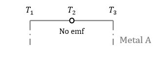
As discussing each type, we can infer two laws of thermocouples: The first law is the law of homogeneous metals. The law states that if a thermocouple is made of the same material, emf is not generated, even if there is a temperature difference.
(Figure 4.3)
The second is the law of intermediate metals. The law states that when a third metal is interposed between two metals and the temperature at the junctions are the same, the third metal cannot affect the net emf.

(Figure 4.4)
Cold junction compensation
When measuring the emf for each type based on temperature, we set the cold junction at 0°C. To use the data in tables or graphs, we should maintain the cold junction at 0°C, but it is not easy to achieve in practice. Therefore, for convenience, we set a reference temperature other than 0°C. According to the law of intermediate temperatures, we use (Eq 4.6) to compensate for the deviation from 0°C.
\( {\small\displaystyle\begin{align} E\left(T_h,T_0\right) \quad&=\quad E\left(T_h,T_r\right)\,+\,E\left(T_r,T_0\right) \tag{Eq 4.6} \end{align} } \)
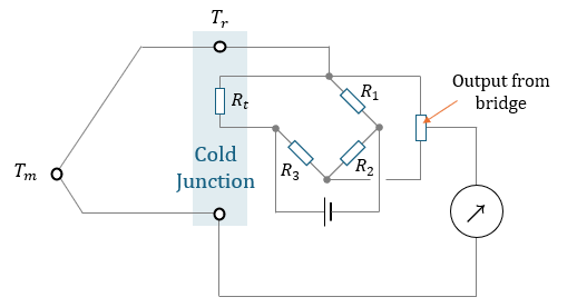
We can incorporate several elements into the existing circuit to automatically calculate cold junction compensation. (Figure 4.4) shows the addition of a Wheatstone bridge with a resistance thermometer, \({\small\displaystyle R_t}\). The bridge is stable at 0°C. The resistance changes when the cold junction deviates from 0°C, resulting in a measurable voltage. The output voltage of the bridge corresponds to \({\small\displaystyle E(T_r,\,T_0)}\). Therefore, the voltage measured by the indicator is \({\small\displaystyle E(T_h,\,T_0)}\) according to (Eq 4.6).
(Figure 4.5)
According to (Eq 3.2), the resistance change of the resistance thermometer is
\( {\small\displaystyle\begin{align} \delta R_t \,=\, R_0(1\,+\,\alpha T)\,-\,R_0 \,=\, R_0\alpha T \tag*{} \end{align} } \)
, and the voltage change of the bridge is:
\( {\small\displaystyle\begin{align} V_0 \quad&=\quad V_s\left(\frac{R_t}{R_t\,+\,R_1}\,-\,\frac{R_3}{R_2\,+\,R_3}\right) \\[10pt] \delta V_0 \quad&=\quad V_s\left(\frac{\delta R_t}{R_0\,+\,\delta R_t\,+\,R_1}\right) \\[10pt] &\approx\quad V_s\left(\frac{\delta R_t}{R_0\,+\,R_1}\right) \,=\, \frac{V_sR_0\alpha T}{R_0\,+\,R_1} \tag*{} \end{align} } \)
Therfore, we obtain (Eq 4.7).
\( {\small\displaystyle\begin{align} E(T_r,\,T_0) \quad=\quad \frac{V_sR_0\alpha T}{R_0\,+\,R_1} \tag{Eq 4.7} \end{align} } \)
3. Junction types of thermocouple
Temperature measurements may require fast response times or contamination protection. When choosing sheathed thermocouple thermometers, we need to select the junction type for the thermocouple thermometer based on the situation. There are three main types: Ungrounded, Grounded, and Exposed type.

(Figure 4.6)
- Ungrounded junction
The sheath and the sensing element are separated. This type provides electromagnetic shielding isolation but has a low response time.
- Grounded junction
In this type, the sensor element is in contact with the sheath. So, the response time is faster compared to the ungrounded junction type.
- Exposed junction
The sensor is exposed, resulting in a fast response time, but it is not protected. Consequently, its lifespan is relatively short compared to other types, limiting their usage environments.
Nomenclature
\({\small\displaystyle E}\) : emf(electr0motive force)
\({\small\displaystyle R}\) : resistance
\({\small\displaystyle S_i}\) : absolute Seebeck coefficient
\({\small\displaystyle S_{AB}}\) : relative Seebeck coefficient
\({\small\displaystyle T}\) : temperature
\({\small\displaystyle V}\) : voltage