
Episode 01. Mass Balance without Reaction
Summary
In this episode, we introduce mass (or material) balance. Mass balance is one of the basic stages of plant design. And it can be utilized in various situation. Therefore, it helps when you enjoy other contents. This episode presents the principle of mass balance and how to calculate it with an example.
1. Introduction
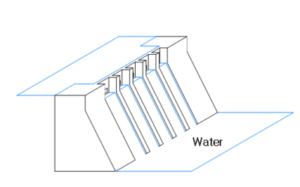
We can find concept of mass balance in life. Let’s think about dam. A dam artificially blocks the flow of water to create a kind of lake. There is incoming flow from upstream or rainwater and outcoming flow through sluice gates. Depending on situations, the gates are opened or closed to adjust water level. This is one of “Mass Balance”.
Mass balance seems simple, but it is a really important step in engineering. It affects several things like pipe, equipment, etc… If mass balance is changed, maybe you will change and repeat your engineering work. Therefore, be careful not to make errors about mass balance.
2. Principle of mass balance
Mass (or material) balance is an application of “law of conservation mass”.
Law of conservation mass
The system’s mass cannot change (no added or no removed), so the quantity is constant over time.
Since the mass does not change, ther must be a balance between input flow, output flow and accumulation. This is summerized as follows (Eq 1.1).
\( {\small\displaystyle\begin{align} i_{in}\,-\,i_{out}\,+\,i_{generation} \quad=\quad i_{accumulation} \tag{Eq 1.1} \end{align} } \)
In (Eq 1.1), there is \({\small\displaystyle i_{generation}}\). What is this? This value is considered about reaction. If composition \({\small\displaystyle i}\) is consumed in a reaction process. In the opposite situation(\({\small\displaystyle i}\) is generated), the value becomes plus.
Think again about the dam. Normally, there is no reaction, so the value of generation is zero. If a precipitation (input flow) is larger than output flow, the water level will gradually rise. In other words, \({\small\displaystyle i_{accumulation}}\) is plus.
3. How to calculate "mass balance without reaction"?
Mass balance can be calculated in various ways depending on point of view like 1) total mass of flow, 2) mass of composition, 3) system. Using these things, you can make several equations and predict about flow what you want to know.
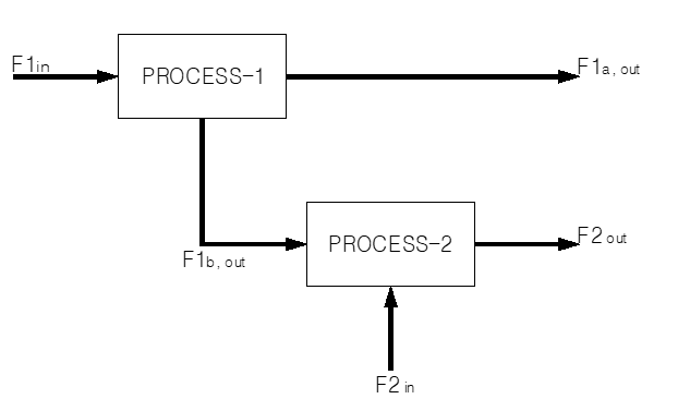
(Figure 1.1)
Let’s see the (Figure 1.1). Input is flow \({\small\displaystyle F_{1,in}}\), and output are flow \({\small\displaystyle F_{1a,out}}\) and \({\small\displaystyle F_{1b,out}}\) in PROCESS-1. In PROCESS-2, \({\small\displaystyle F_{1b,out}}\) and \({\small\displaystyle F_{2,in}}\)are input flows. The output flow is \({\small\displaystyle F_{2,out}}\). All the flows consist of composition \({\small\displaystyle x}\) and \({\small\displaystyle y}\). Some flow’s mass flowrate and composition data are shown in (Table 1.1).
| Flow | \( {\small\displaystyle F_{1,in} } \) | \( {\small\displaystyle F_{1a,out} } \) | \( {\small\displaystyle F_{2,in} } \) |
|---|---|---|---|
| \( {\small\displaystyle \text{Flowrate }[kg/hr] } \) | \( {\small\displaystyle 10,000 } \) | \( {\small\displaystyle 3,000 } \) | \( {\small\displaystyle 3,000 } \) |
| Composition [mass fraction] | |||
| \( {\small\displaystyle x } \) | \( {\small\displaystyle 0.5 } \) | \( {\small\displaystyle 0.85 } \) | \( {\small\displaystyle 0 } \) |
| \( {\small\displaystyle y } \) | \( {\small\displaystyle 0.5 } \) | \( {\small\displaystyle 0.15} \) | \( {\small\displaystyle 1 } \) |
| \( {\small\displaystyle \text{Total} } \) | \( {\small\displaystyle 1 } \) | \( {\small\displaystyle 1 } \) | \( {\small\displaystyle 1 } \) |
In (Figure 1.1), We can set three systems like (Figure 1.2)
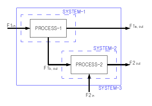
(Figure 1.2)
Assume all systems are steady system and no reaction. The value of \({\small\displaystyle i_{generation}}\) and \({\small\displaystyle i_{accumulation}}\) becomes zero. So, (Eq 1.1) can be changed like below.
\( {\small\displaystyle\begin{align} i_{in}\,-\,i_{out} \quad=\quad 0 \tag{Eq 1.2} \end{align} } \)
Let arrange the equation to tables. (Table 1.2) shows about total flowrate each system. And (Table 1.3) shows about flowrate of composition \({\small\displaystyle x}\) each system.
| Total mass flow | \( {\small\displaystyle i_{in} } \) | \( {\small\displaystyle i_{out} } \) | \( {\small\displaystyle i_{in} \,-\, i_{out} \quad=\quad 0 } \) |
|---|---|---|---|
| System - 1 | \( {\small\displaystyle F_{1,in} } \) | \( {\small\displaystyle\begin{align} F_{1a,out} \\[10pt] F_{1b,out} \end{align} } \) | \( {\small\displaystyle F_{1,in}\,-\,\left(F_{1a,out}\,+\,F_{1b,out}\right) \quad=\quad 0 } \) |
| System - 2 | \( {\small\displaystyle\begin{align} F_{1b,out} \\[10pt] F_{2,in} \end{align} } \) | \( {\small\displaystyle F_{2,out} } \) | \( {\small\displaystyle \left(F_{1b,out}\,+\,F_{2,in}\right)\,-\,F_{2,out} \quad=\quad 0 } \) |
| System - 3 | \( {\small\displaystyle\begin{align} F_{1,in} \\[10pt] F_{2,in} \end{align} } \) | \( {\small\displaystyle\begin{align} F_{1a,out} \\[10pt] F_{2,out} \end{align} } \) | \( {\small\displaystyle \left(F_{1,in}\,+\,F_{2,in}\right)\,-\,\left(F_{1a,out}\,+\,F_{2,out}\right) \quad=\quad 0 } \) |
| \( {\small\displaystyle \text{Composition }x } \) | \( {\small\displaystyle i_{in} } \) | \( {\small\displaystyle i_{out} } \) | \( {\small\displaystyle i_{in}\,-\,i_{out} } \quad=\quad 0 \) |
|---|---|---|---|
| System - 1 | \( {\small\displaystyle 0.5F_{1,in} } \) | \( {\small\displaystyle\begin{gather} 0.85F_{1a,out} \\[10pt] x_{1b,out}F_{1b,out} \end{gather} } \) | \( {\small\displaystyle 0.5F_{1,in}\,-\,\left(0.85F_{1a,out}\,+\,x_{1b,out}F_{1b,out}\right) \quad=\quad 0 } \) |
| System - 2 | \( {\small\displaystyle x_{1b,out} F_{1b,out} } \) | \( {\small\displaystyle x_{2,out} F_{2,out} } \) | \( {\small\displaystyle x_{1b,out} F_{1b,out} \,-\,x_{2,out}F_{2,out} \quad=\quad 0 } \) |
| System - 3 | \( {\small\displaystyle 0.5 F_{1,in} } \) | \( {\small\displaystyle\begin{gather} 0.85 F_{1a,out} \\[10pt] x_{2,out}F_{2,out} \end{gather} } \) | \( {\small\displaystyle 0.5 F_{1,in}\,-\, \left(0.85F_{1a,out}\,+\,x_{2,out}F_{2,out}\right) \quad=\quad 0 } \) |
We already know the flowrate data about \({\small\displaystyle F_{1,in},\,F_{1a,out}}\), and \({\small\displaystyle F_{2,in}}\). So we can solve above equations in the tables. The result is in (table 1.4).
| Flow | \( {\small\displaystyle F_{1,in} } \) | \( {\small\displaystyle F_{1a,out} } \) | \( {\small\displaystyle F_{1b,out} } \) | \( {\small\displaystyle F_{2,in} } \) | \( {\small\displaystyle F_{2,out} } \) |
|---|---|---|---|---|---|
| \( {\small\displaystyle \text{Flowrate }[kg/hr] } \) | \( {\small\displaystyle 10,000 } \) | \( {\small\displaystyle 3,000 } \) | \( {\small\displaystyle 7,000 } \) | \( {\small\displaystyle 3,000 } \) | \( {\small\displaystyle 10,000 } \) |
| Composition [mass fraction] | |||||
| \( {\small\displaystyle x } \) | \( {\small\displaystyle 0.5 } \) | \( {\small\displaystyle 0.85 } \) | \( {\small\displaystyle 0.35 } \) | \( {\small\displaystyle 0 } \) | \( {\small\displaystyle 0.245 } \) |
| \( {\small\displaystyle y } \) | \( {\small\displaystyle 0.5 } \) | \( {\small\displaystyle 0.15 } \) | \( {\small\displaystyle 0.65 } \) | \( {\small\displaystyle 1 } \) | \( {\small\displaystyle 0.755 } \) |
| \( {\small\displaystyle \text{Total} } \) | \( {\small\displaystyle 1 } \) | \( {\small\displaystyle 1 } \) | \( {\small\displaystyle 1 } \) | \( {\small\displaystyle 1 } \) | \( {\small\displaystyle 1 } \) |
Of course, maybe it is not simple like above example in real. A system can have reaction, more various inlet, or outlet. However, if you understand principle of mass balance and how to calculate it, you can make or analysis like the example in any situations.