Episode 03. Criteria for Equilibrium and Phase Equilibrium
Summary
Equilibrium is a crucial thermodynamic concept, representing a state where there is no change over time when observed on a macroscopic scale. In this episode, we cover the equilibrium criteria based on different systems. Finally, we discuss the properties of a closed system (given temperature and pressure) at phase equilibrium.
1. Introduction
Equilibrium is a significant concept since it acts as an indicator for determining how a given system will progress. Then, what is the “Equilibrium”? Equilibrium can be described as a state in which there is no change over time in the system when observed macroscopically.
In this episode, we discuss the equilibrium criteria and the behavior of properties in various phases of a specific system when they coexist in equilibrium. To determine the equilibrium state, we utilize the 1st and 2nd laws of thermodynamics covered in Episode 01. (For convenience, the total mole number in (Eq 1.10) is considered as 1.)
\( {\small\displaystyle\begin{align} dU_{system} \quad&=\quad dQ_{rev}\,+\,dW_{rev} \tag{Eq 1.10} \\[15pt] ∆S_t \quad&\ge\quad 0 \tag{Eq 1.3} \\[15pt] dS_{system} \quad&=\quad \frac{dQ_{rev}}{T} \tag{Eq 1.4} \end{align} } \)
We can express the total entropy change as the combination of the entropy changes within the system and those of the surroundings. Furthermore, because of reversible heat exchange, the heat of the system and its surroundings differs only in direction, while their magnitudes are the same.
\( {\small\displaystyle\begin{align} dS_t \quad&=\quad dS_{system} \,+\, dS_{surr} \\[15pt] \frac{dQ_{rev}}{T} \quad&=\quad -\frac{dQ_{surr}}{T_{surr}} \tag*{} \end{align} } \)
Combining these characteristics with the 2nd law of thermodynamics, we can express it as (Eq 3.1). Now, let’s discuss the equilibrium criteria for various systems.
\( {\small\displaystyle\begin{align} dS_{system} \,+\, dS_{surr} \quad&\ge\quad 0 \\[15pt] dS_{system} \quad&\ge\quad \frac{dQ_{rev}}{T} \tag{Eq 3.1} \end{align} } \)
2. Equilibrium criteria for various systems
Case 1 : Isolated system – Constant volume
Since there is no heat exchange with the surroundings and the system’s volume is constant, the terms of the heat and work in (Eq 1.10) become zero. It implies the internal energy(U) of the system remains constant. Additionally, the right side of (Eq 3.1) equates to zero, indicating that the differential change in entropy of the system is always greater than or equal to zero.
\( {\small\displaystyle\begin{align} dU_{system} \,=\, 0 \quad&\longrightarrow\quad U \,=\, \text{constant} \\[15pt] dS_{system} \,\ge\, \frac{dQ_{rev}}{T} \quad&\longrightarrow\quad dS_{system} \,\ge\, 0 \tag*{} \end{align} } \)
Looking at the equation above, it becomes evident that the entropy only increases until the system reaches the equilibrium state. And the equilibrium criterion for the system is when the term of dSsystem becomes zero, precisely when the system’s entropy becomes its maximum value.
Case 2 : Closed system – Constant volume, Constant temperature
In this case, where volume remains constant and only heat exchange exists, we can simplify (Eq 1.10) as follows. Furthermore, we can understand that the differential change in internal energy is not more than \({\small\displaystyle TdS}\) by utilizing (Eq 3.1).
\( {\small\displaystyle\begin{align} dU_{system} \quad&=\quad dQ_{rev} \\[15pt] dU_{system} \quad&\le\quad TdS_{system} \tag*{} \end{align} } \)
Then, we set the right side of the equation to 0. Since the temperature is constant, we can rearrange it as follows.
\( {\small\displaystyle\begin{align} dU_{system} \,-\, TdS_{system} \quad&\le\quad 0 \\[15pt] d(U\,-\,TS)_{system} \quad&\le\quad 0 \tag*{} \end{align} } \)
Based on (Eq 1.8), we can express the above equation in terms of the Helmholtz free energy.
\( {\small\displaystyle\begin{align} dA_{system} \quad\le\quad 0 \tag*{} \end{align} } \)
Until the system reaches equilibrium, the Helmholtz free energy of the system only decreases. As a result, the equilibrium criterion for the system is when the differential change in Helmholtz free energy becomes zero – precisely when the Helmholtz free energy reaches its minimum value.
Case 3 : Closed system – Constant temperature, Constant pressure
In the third case, where both heat and work are present, we use (Eq 1.10) as it stands. Let’s rearrange the heat term in (Eq 1.10) on the left side and the remaining terms on the right.
\( {\small\displaystyle\begin{align} dQ_{system} \quad=\quad dU_{system} \,-\, dW_{rev} \tag*{} \end{align} } \)
By using (Eq 3.1), we can confirm that the equation is not more than TdS, and due to constant temperature and pressure, we can arrange it as follows.
\( {\small\displaystyle\begin{align} dU_{system}\,-\,dW_{rev} \quad&\le\quad TdS_{system} \\[15pt] dU_{system}\,+\,PdV\,-\,TdS_{system} \quad&\le\quad 0 \\[15pt] d(U\,+\,PV\,-\,TS)_{system} \quad&\le\quad 0 \tag*{} \end{align} } \)
Through (Eq 1.7) and (Eq 1.9), we can represent the above equation in terms of Gibbs free energy.
\( {\small\displaystyle\begin{align} dG_{system} \quad\le\quad 0 \tag*{} \end{align} } \)
Until the system reaches an equilibrium state, the Gibbs free energy of the system only decreases. The equilibrium criterion for the system is when the differential change in Gibbs free energy becomes zero – precisely when the Gibbs free energy reaches its minimum value at the given temperature and pressure.
3. Phase equilibrium
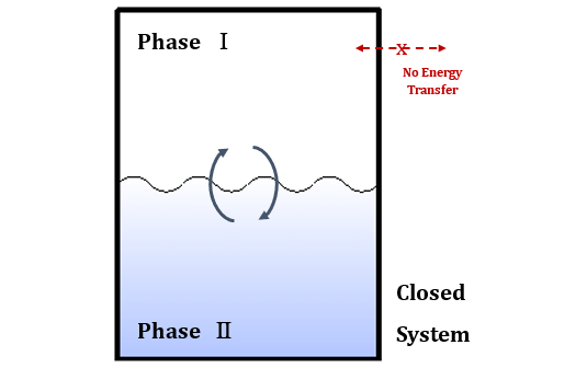
Case 3 is a system frequently encountered. Now, we discuss phase equilibrium within a Case 3 system which has multiple phases. Let’s take a look at (Figure 3.1) below.

(Figure 3.1)
Two distinct phases (Ⅰ and Ⅱ) are present in (Figure 3.1). Each phase can exchange material and heat with the other, and the total system satisfies the same conditions as Case 3. If the two phases are at equilibrium, what characteristics will they fulfill? (Assuming no chemical reactions.) By utilizing (Eq 1.24), we can arrange differential changes in the Gibbs free energy of each phase.
\( {\small\displaystyle\begin{align} \text{Phase }\mathrm{I} \,:\, d(nG)^{\mathrm{I}} \quad&=\quad (nV)^{\mathrm{I}}dP\,-\,(nS)^{\mathrm{I}}dT\,+\,\sum_i \mu_i^{\mathrm{I}}\,dn_i^{\mathrm{I}} \\[15pt] \text{Phase }\mathrm{II} \,:\, d(nG)^{\mathrm{II}} \quad&=\quad (nV)^{\mathrm{II}}dP\,-\,(nS)^{\mathrm{II}}dT\,+\,\sum_i \mu_i^{\mathrm{II}}\,dn_i^{\mathrm{II}} \tag*{} \end{align} } \)
We can also express the differential change in total Gibbs free energy can also in a similar way. A key aspect to note here is that due to the total system being a closed system, the \({\small\displaystyle\sum_i\mu_{t,i}dn_{t,i}}\) becomes 0. Additionally, the \({\small\displaystyle\sum_i\mu_{t,i}dn_{t,i}}\) is identical to the sum of the \({\small\displaystyle\sum_i\mu_idn_i}\) of each phase.
\( {\small\displaystyle\begin{gather} d(nG)_t \quad=\quad (nV)_tdP\,-\,(nS)_tdT\,+\,\sum_i \mu_{t,i}\,dn_{t,i}, \qquad \sum_i \mu_{t,i}\,dn_{t,i} \quad=\quad 0 \\[15pt] \sum_i \mu_{t,i}\,dn_{t,i} \quad=\quad \sum_i \mu_i^{\mathrm{I}}\,dn_i^{\mathrm{I}} \,+\, \sum_i \mu_i^{\mathrm{II}}\,dn_i^{\mathrm{II}} \tag*{} \end{gather} } \)
The mole number in the two phases interacts with each other. In other words, when the mole number of a specific component in Phase Ⅰ decreases, the mole number of the component in Phase Ⅱ increases by the same amount. Based on this, we can confirm that the chemical potentials of each phase are identical. Expanding this concept, we can express it as shown in (Eq 3.2).
\( {\small\displaystyle\begin{gather} dn_i^{\mathrm{I}} \quad=\quad -dn_i^{\mathrm{II}} \\[15pt] \sum_i \left(\mu_i^{\mathrm{I}}\,-\,\mu_i^{\mathrm{II}}\right)\,dn_i^{\mathrm{I}} \quad=\quad 0 \quad\longrightarrow\quad \mu_i^{\mathrm{I}} \quad=\quad \mu_i^{\mathrm{II}} \\[15pt] \mu_i^{\mathrm{I}} \,=\, \mu_i^{\mathrm{II}} \,=\, \mu_i^{\mathrm{III}} \,=\, \quad\cdots\quad \,=\, \mu_i^{\theta} \tag{Eq 3.2} \end{gather} } \)
Properties of pure species at phase equilibrium
Let’s assume a situation where pure species coexist in two phases (Ⅰ and Ⅱ) at an equilibrium state. According to (Eq 3.2), the chemical potentials of pure species i in both phases are equal. And since the system consists of pure species, nt and ni in each phase are the same. Consequently, we can derive that when pure species reach equilibrium, the Gibbs free energy of each phase becomes identical.
\( {\small\displaystyle\begin{gather} \mu_i^{\mathrm{I}} \quad=\quad \mu_i^{\mathrm{II}} \quad\longrightarrow\quad \left[\frac{\partial \left(n^{\mathrm{I}}G^{\mathrm{I}}\right)}{\partial n_i^{\mathrm{I}}}\right]_{T,P,n_i^{\mathrm{II}}} \quad=\quad \left[\frac{\partial \left(n^{\mathrm{II}}G^{\mathrm{II}}\right)}{\partial n_i^{\mathrm{II}}}\right]_{T,P,n_i^{\mathrm{I}}} \tag*{} \end{gather} } \)
\( {\small\displaystyle\begin{align} G_i^{\mathrm{I}} \quad=\quad G_i^{\mathrm{II}} \tag{Eq 3.3} \end{align} } \)
Based on (Eq 2.10), we can express the Gibbs free energy of the pure species in each phase as follows. Through the equations about Gibbs free energy and (Eq 3.3), we can conclude that if both phases are in equilibrium, the fugacity of the pure species existing in each phase is also identical.
\( {\small\displaystyle\begin{align} \text{Phase }\mathrm{I} \,:\, G_i^{\mathrm{I}}(T,P) \quad&=\quad g(T)\,+\,RTlnf_i^{\mathrm{I}} \\[15pt] \text{Phase }\mathrm{II} \,:\, G_i^{\mathrm{II}}(T,P) \quad&=\quad g(T)\,+\,RTlnf_i^{\mathrm{II}} \tag*{} \end{align} } \)
\( {\small\displaystyle\begin{gather} G_i^{\mathrm{I}} \,=\, G_i^{\mathrm{II}} \quad\longrightarrow\quad f_i^{\mathrm{I}} \,=\, f_i^{\mathrm{II}} \\[15pt] f_i^{\mathrm{I}} \,=\, f_i^{\mathrm{II}} \,=\, f_i^{\mathrm{III}} \,=\, \quad\cdots\quad \,=\, f_i^{\theta} \tag{Eq 3.4} \end{gather} } \)
Let’s consider that the pure species exists in both the gas and liquid phases. If the pure species are in phase equilibrium, we can deduce that it is in a saturated state. In other words, the pressure is equal to the vapor pressure of the species at the given temperature. By applying this, we can derive the following relationships.
\( {\small\displaystyle\begin{align} P \quad&=\quad P_i^{sat} \\[15pt] f_i^v\,=\,f_i^l\,=\,f_i^{sat} \quad&=\quad \phi_i^{sat}P_i^{sat} \tag{Eq 3.5} \\[15pt] \phi_i^v\,=\,\phi_i^l\,=\,\phi_i^{sat} \quad&=\quad \frac{f_i^{sat}}{P_i^{sat}} \tag{Eq 3.6} \end{align} } \)
Properties of a component in mixtures at phase equilibrium
Now, let’s discuss the phase equilibrium of a mixture. Do you remember that we defined the chemical potential using an expression involving fugacity in Episode 02? If a mixture coexists in two different phases as shown in (Figure 3.1), we can express the \({\small\displaystyle\mu_i}\) of each phase using (Eq 2.14)
\( {\small\displaystyle\begin{align} \text{Phase }\mathrm{I} \,:\, \mu_i^{\mathrm{I}} \quad&=\quad g(T)\,+\,RTln\hat{f_i}^{\mathrm{I}} \\[15pt] \text{Phase }\mathrm{II} \,:\, \mu_i^{\mathrm{II}} \quad&=\quad g(T)\,+\,RTln\hat{f_i}^{\mathrm{II}} \tag*{} \end{align} } \)
When two phases reach the equilibrium state, we can derive from (Eq 3.2) that the \({\small\displaystyle\hat{f_i}}\) of each phase is equal. Expanding this concept, it becomes (Eq 3.7).
\( {\small\displaystyle\begin{gather} \mu_i^{\mathrm{I}} \,=\, \mu_i^{\mathrm{II}} \quad\longrightarrow\quad \hat{f_i}^{\mathrm{I}} \,=\, \hat{f_i}^{\mathrm{II}} \\[15pt] \hat{f_i}^{\mathrm{I}} \,=\, \hat{f_i}^{\mathrm{II}} \,=\, \hat{f_i}^{\mathrm{III}} \,=\, \quad\cdots\quad \,=\, \hat{f_i}^{\theta} \tag{Eq 3.7} \end{gather} } \)
Nomenclature
\({\small\displaystyle A}\) : Helmholtz free energy
\({\small\displaystyle f}\) : fugacity
\({\small\displaystyle G}\) : Gibbs free energy
\({\small\displaystyle n}\) : mole number
\({\small\displaystyle P}\) : pressure
\({\small\displaystyle P_i^{sat}}\) : vapor pressure of pure species
\({\small\displaystyle Q}\) : heat
\({\small\displaystyle S}\) : entropy
\({\small\displaystyle T}\) : temperature
\({\small\displaystyle U}\) : internal energy
\({\small\displaystyle V}\) : volume
\({\small\displaystyle W}\) : work
\({\small\displaystyle\mu}\) : chemical potential
\({\small\displaystyle\phi}\) : fugacity coefficient