Episode 06. Liquid - Liquid Equilibrium
Summary
Liquid mixtures can exist in a single phase. However, they may also separate into multiple liquid phases. This episode covers liquid-liquid phase equilibrium under constant temperature and pressure. First, we determine the conditions for liquid-liquid phase equilibrium using fugacity. We then examine the Gibbs free energy behavior in phase equilibrium.
1. Introduction
Some liquid mixtures, such as water and ethanol, form a single phase, whereas others, such as water and oil, separate into two immiscible liquid phases. Then, when does phase separation occur, and how can we determine the equilibrium conditions during phase separation?
In this episode, we discuss phase equilibrium for mixtures that form liquid-liquid phases and analyze them in terms of Gibbs free energy. For simplicity, we assume a binary system.

(Figure 6.1)
2. Liquid - Liquid equilibrium in closed system
Consider two liquid phases, \({\small\displaystyle \text{I}}\) and \({\small\displaystyle \text{II}}\). As discussed in Episode 02, the fugacity of a given component is identical in both phases. Furthermore, based on (Eq 2.18), this relationship can be expressed as (Eq 6.1).
\( {\small\displaystyle\begin{align} \hat{f}_i^{\text{I}} \quad&=\quad \hat{f}_i^{\text{II}} \\[15pt] x_i^{\text{I}}\gamma_i^{\text{I}}f_i^{\text{I}} \quad&=\quad x_i^{\text{II}}\gamma_i^{\text{II}}f_i^{\text{II}} \tag{Eq 6.1} \end{align} } \)
Since the fugacity of a pure substance is equal in both phases when the system is in equilibrium, (Eq 6.1) can be rewritten as (Eq 6.2).
\( {\small\displaystyle\begin{align} x_i^{\text{I}}\gamma_i^{\text{I}} \quad&=\quad x_i^{\text{II}}\gamma_i^{\text{II}} \tag{Eq 6.2} \end{align} } \)
The activity coefficients in (Eq 6.2) can be determined using various activity coefficient models. As an example, we can illustrate this using the Margules activity model. The Margules activity model for a binary system is formulated as follows:
\( {\small\displaystyle\begin{align} \frac{\bar{G}^E}{RT} \quad&=\quad \left(A_{12}x_1\,+\,A_{21}x_2\right)x_1x_2 \tag{Eq 6.3} \\[15pt] &=\quad Ax_1x_2 \tag{Eq 6.4} \\[10pt] &\qquad\text{where } A_{12}\,=\,A_{21}\,=\,A \end{align} } \)
(Eq 6.4) is referred to as the one-constant Margules equation. Based on this equation, we can derive the activity coefficients of each component \({\small\displaystyle i}\). Multiplying both sides by \({\small\displaystyle n}\), we obtain:
\( {\small\displaystyle\begin{align} \frac{n\bar{G}^E}{RT} \quad&=\quad A\left(\frac{n_1n_2}{n_1\,+\,n_2}\right) \tag*{} \end{align} } \)
Subsequently, take the partial derivative with respect to \({\small\displaystyle n_1}\)
\( {\small\displaystyle\begin{align} \left[\frac{\partial(n\bar{G}^E/RT)}{\partial n_1}\right] \quad&=\quad A\left(\frac{n_2}{n_1\,+\,n_2}\,-\,\frac{n_1n_2}{(n_1\,+\,n_2)^2}\right) \\[10pt] &=\quad Ax_2^2 \tag{Eq 6.5} \end{align} } \)
Next, we can calculate the values of the activity coefficients by applying (Eq 2.18).
\( {\small\displaystyle\begin{align} \ln \gamma_1 \,=\, Ax_2^2 \quad\longrightarrow\quad \gamma_1 \,=\, \exp (Ax_2^2) \\[15pt] \ln \gamma_2 \,=\, Ax_1^2 \quad\longrightarrow\quad \gamma_2 \,=\, \exp (Ax_1^2) \tag*{} \end{align} } \)
Therefore, using the Margules activity model, we can derive an expression for liquid-liquid equilibrium (LLE) as follows:
\( {\small\displaystyle\begin{align} x_1^{\text{I}}\exp\left[A(1\,-\,x_1^{\text{I}})^2\right] \quad=\quad x_1^{\text{II}}\exp\left[A(1\,-\,x_1^{\text{II}})^2\right] \tag{Eq 6.6} \end{align} } \)
3.Gibbs free energy in LLE
Next, we examine the Gibbs free energy of liquid-liquid mixtures. As discussed in Episode 03, under constant pressure and temperature, the total Gibbs Free energy of the system tends to decrease. The Gibbs free energy of a real liquid mixture is the sum of the Gibbs free energy of an ideal solution and the excess Gibbs free energy.
\( {\small\displaystyle\begin{align} G \quad=\quad G^{id}\,+\,G^E \tag*{} \end{align} } \)
For a binary system, this equation can be rearranged using (Eq 2.1) and (Eq 2.16) as follows:
\( {\small\displaystyle\begin{align} G^{id} \quad&=\quad \sum_i\,x_i\bar{G}_i^{id} \\[15pt] G \quad&=\quad x_1G_1\,+\,x_2G_2\,+\,RT(x_1\ln x_1\,+\,x_2\ln x_2)\,+\,G^E \tag{Eq 6.7} \\[15pt] \frac{\Delta G}{RT} \quad&=\quad x_1\ln x_1\,+\,x_2\ln x_2\,+\,\frac{G^E}{RT} \tag{Eq 6.8} \\[10pt] &\qquad \text{where }\Delta G\,=\,G\,-\,\sum_i\,x_iG_i \end{align} } \)
Since a system becomes more stable as Gibbs free energy decreases, \({\small\displaystyle \Delta G}\) is negative. Under constant temperature and pressure, a system should satisfy \({\small\displaystyle \partial^2\left(\Delta G\right)\,>\,0}\) to remain a single-phase state. As shown in (Figure 6.2), if this value is negative, the system is thermodynamically more stable when it separates into two phases.

(Figure 6.2)
\( {\small\displaystyle\begin{align} \frac{\partial^2(\Delta G/RT)}{\partial x_1^2} \quad>\quad 0 \tag{Eq 6.9} \end{align} } \)
Taking the second derivative of (Eq 6.9) gives:
\( {\small\displaystyle\begin{align} \frac{\partial^2(\Delta G/RT)}{\partial x_1^2} \quad=\quad \frac{1}{x_1x_2} \,+\, \frac{\partial^2(G^E/RT)}{\partial x_1^2} \tag{Eq 6.10} \end{align} } \)
Therefore, to maintain a single-phase state, the system must satisfy the following conditions:
\( {\small\displaystyle\begin{align} \frac{\partial^2(G^E/RT)}{\partial x_1^2} \quad>\quad -\frac{1}{x_1x_2} \tag{Eq 6.11} \end{align} } \)
Let’s rearrange this relationship using the one constant Margules equation.
\( {\small\displaystyle\begin{align} \frac{\partial^2(G^E/RT)}{\partial x_1^2} \quad&=\quad -2A \\[15pt] T \quad&>\quad \frac{2Ax_1x_2}{R} \tag{Eq 6.12} \end{align} } \)
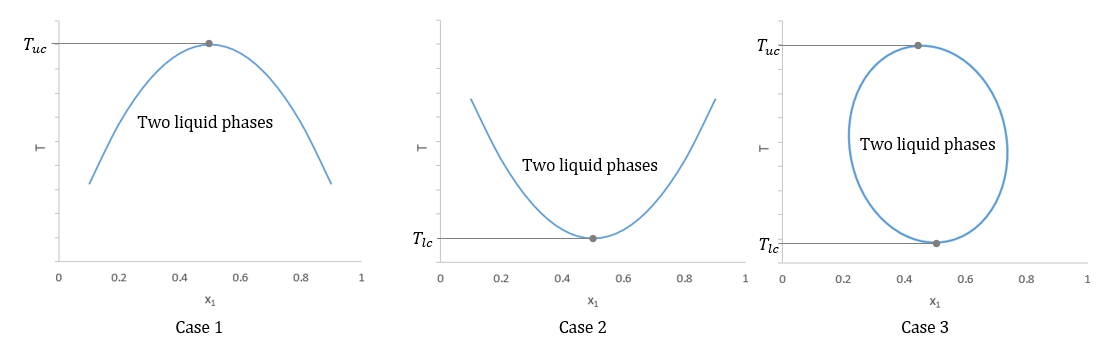
If the temperature satisfies (Eq 6.12), the mixture exists as a single phase; otherwise, phase separation occurs. As shown in (Figure 6.3), the phase behavior of the mixture changes as a function of temperature, with multiple possible cases.
(Figure 6.3)
In (Figure 6.3), \({\small\displaystyle T_{uc}}\) and \({\small\displaystyle T_{lc}}\) represent the upper and lower consolute temperatures, also known as the upper and lower critical solution temperatures (UCST and LCST), respectively. For \({\small\displaystyle T\,>\,T_{uc}}\) or \({\small\displaystyle T\,<\,T_{lc}}\), the system remains in a single liquid phase across all compositions. However, when \({\small\displaystyle T_{lc}\,<\,T\,<\,T_{uc}}\), liquid phase separation can occur. Note that the Margules equation (if \({\small\displaystyle A>0}\)) can be used solely to determine the value of \({\small\displaystyle T_{uc}}\), implying that only the corresponding graph for Case 1 can be obtained.
Nomenclature
\({\small\displaystyle A}\) : Margules activity model parameter
\({\small\displaystyle f_i}\) : fugacity of pure species i
\({\small\displaystyle \hat{f}_i}\) : fugacity of component i in mixtures
\({\small\displaystyle G}\) : Gibbs free energy
\({\small\displaystyle \bar{G}}\) : partial molar Gibbs free energy
\({\small\displaystyle G^{id}}\) : ideal solution Gibbs free energy
\({\small\displaystyle G^{e}}\) : excess Gibbs free energy
\({\small\displaystyle n_i}\) : moles of component i
\({\small\displaystyle R}\) : gas constant
\({\small\displaystyle T}\) : temperature
\({\small\displaystyle x_i}\) : mole fraction of component i
\({\small\displaystyle \gamma}\) : activity coefficient