Episode 03. Heat Balance Without Reaction
Summary
We need to know the amount of energy required for operation. Then, how to know it? We can calculate how much the cooling and heating medium, fuel, etc. is needed through heat (or energy) balance. So, it is an important step. In this episode, we introduce heat (or energy) balance without reaction and how to calculate it through an example.
1. Introduction
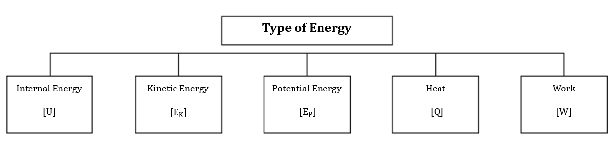
(Figure 3.1)
Let’s assume that there are temperature conditions required for product production. So how much heating or cooling medium is needed to reach this temperature? To know this, we have to calculate the heat (or energy) balance. We can find the required energy for operating the equipment or the entire plant from heat (or energy) balance. Therefore, Heat (or energy) balance is also significant in engineering. However, because energy exists in many forms (Figure 3.1), it is more complex than the mass balance. To avoid confusion of terminology, we will express it as energy balance rather than heat balance.
2. Energy balance without reaction
The energy balance can be divided into without reaction and with reaction cases. First, we look into energy balance without reaction. As with the mass balance, we utilize (Eq 1.1) from Mass & Heat Balance Episode 01.
\( {\small\displaystyle\begin{align} i_{in} \,-\, i_{out} \,+\, i_{generation} \quad=\quad i_{accumulation} \tag{Eq 1.1} \end{align} } \)
Since there is no reaction, igeneration becomes zero. However, since energy exists in various types, we need to consider these terms additionally. First, a fluid has internal(U), kinetic (EK), and potential (EP) energy. And there is heat and work which is entering or leaving the system. Finally, we consider the flow work perfomed when a fluid enters and exits the system. So, the equation can change to (Eq 3.1).
\( {\small\displaystyle\begin{matrix} \underbrace{(U_{in}\,+\,E_{K, in}\,+\,E_{P,in})}_{i_{in}} \,-\, \underbrace{(U_{out}\,+\,E_{K, out}\,+\,E_{P,out})}_{i_{out}} \,+\, \underbrace{Q}_{\text{Net Heat}} \,+\, \underbrace{W}_{\text{Net Work}} \,+\, \underbrace{P_{in}V_{in}\,-\,P_{out}V_{out}}_{\text{Flow Work}} \quad&=&\quad \underbrace{(U\,+\,E_K\,+\,E_P)_{accumulation}}_{i_{accumulation}} &\text{(Eq 3.1)} \end{matrix} } \)
Heat and work have positive values when they enter the system and negative values when they exit the system. The word “Net” refers to the sum of the incoming and outgoing amounts. By combining the terms of U and PV in (Eq 3.1), it can convert to enthalpy. And if the system is in a gravitational field, the equation can be arranged as (Eq 3.2) or (Eq 3.3).
\( {\small\displaystyle\begin{matrix} (H_{in}\,+\,\frac{1}{2}m_{in}v^2_{in} \,+\,m_{in}gh_{in}) \,-\, (H_{out}\,+\,\frac{1}{2} m_{out}v^2_{out}\,+\,m_{out}gh_{out}) \,+\, Q\,+\,W \quad&=&\quad (U\,+\,E_K\,+\,E_P)_{accumulation} &\quad\text{(Eq 3.2)} \\[15pt] m_{in}(\hat{H}_{in}\,+\, \frac{1}{2}v^2_{in}\,+\, gh_{in})\,-\, m_{out}(\hat{H}_{out} \,+\, \frac{1}{2}v^2_{out}\,+\, gh_{out}) \,+\, Q\,+\,W \quad&=&\quad (U\,+\,E_K\,+\,E_P)_{accumulation} &\quad\text{(Eq 3.3)} \end{matrix} } \)
\( {\small\displaystyle\begin{align} ∵\ H \quad\equiv\quad U\,+\,PV, \quad E_K \quad=\quad \frac{1}{2}mv^2, \quad E_P \quad=\quad mgh\, (\text{In gravitaional field}) \tag*{} \end{align} } \)
Assuming that the pressure is constant, the enthalpy can be expressed as a combination of specific heat capacity and temperature.
\( {\small\displaystyle\begin{matrix} m_{in}\{C_{P,in}(T\,-\,T_{ref})\,+\,\frac{1}{2}v^2_{in}\,+\,gh_{in}\} \,-\, m_{out}\{C_{P,out}(T\,-\,T_{ref})\,+\,\frac{1}{2}v^2_{out}\,+\,gh_{out}\} \,+\, Q\,+\,W \quad&=&\quad (U\,+\,E_K\,+\,E_P)_{accmulation} &\text{(Eq 3.4)} \end{matrix} } \)
\( {\small\displaystyle\begin{align} ∵ \, &\hat{H} \,=\, \hat{H}(T, P) \quad\longrightarrow\quad d\hat{H} \,=\, \left(\partial\hat{H}\over\partial T\right)_PdT\,+\, \left(\partial\hat{H}\over\partial P\right)_TdP \quad\text{and}\quad C_P\equiv \left(\partial\hat{H}\over\partial T\right)_P \\[15pt] &\text{If pressure is constant,} \quad d\hat{H} \,=\, C_PdT \quad\longrightarrow\quad \hat{H} \,=\, \int_{T_{ref}}^{T} C_PdT \\[15pt] &\text{If heat capacity is constant,} \quad \hat{H} \,=\, C_P(T-T_{ref}) \tag*{} \end{align} } \)
3. How to calculate energy balance without reaction?
Do you remember the example in episode 01? (Figure 3.2) adds heat and work to the example calculated in the previous episode. And the specific heat capacity of each flow and the temperature of some flows are shown in (Table 3.1). We will find empty information in (Table 3.1) using (Eq 3.4). Before we do the calculations, let’s make several assumptions.
Assumption
- The systems are steady state
- All flow's v and h are same
- Temperature of outputs from Prcoess -1 is same
- Pressure and Specific heat capacity is constant
- There is no phase change within the range of Tref to T

(Figure 3.2)

(Table 3.1)
Since the system is steady state, the right side of (Eq 3.4) becomes zero. And kinetic energy and potential energy can be omitted by the second assumption. So, (Eq 3.5) can be derived.
\( {\small\displaystyle\begin{align} m_{in}C_{P,in}(T_{in}\,-\,T_{ref}) \,-\, m_{out}{C_{P,out}(T_{out}\,-\,T_{ref})} \,+\, Q\,+\,W \quad=\quad 0 \tag{Eq 3.5} \end{align} } \)
(Figure 3.2) can be divided into system -1 and system -2 shown in (Figure 3.3). We will set the equation for two systems and the total system. The components of (Eq 3.5) for each system and the total system are summarized in (Table 3.2). The temperature of F1a, out and F1b, out is indicated T1, and the temperature of F2, out by T2.
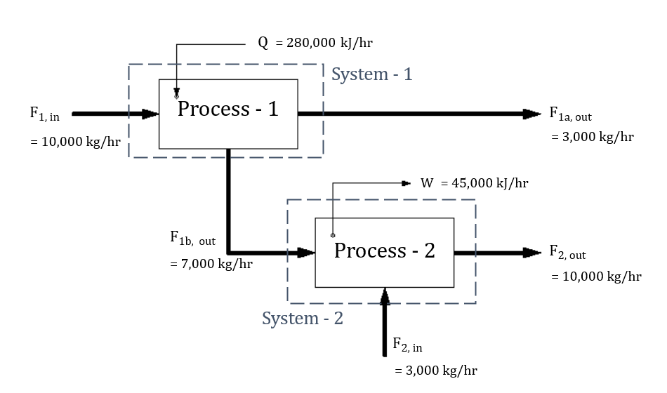
(Figure 3.3)
| System | iin | iout | Q | W |
|---|---|---|---|---|
| System - 1 | F1,in : \( {\small\displaystyle 10,000\frac{kg}{hr}\,\times\,1\frac{kJ}{kg\cdot K}\,\times\,\{(50\,+\,273.15)\,-\,273.15\}K } \) | F1a,out : \( {\small\displaystyle 3,000\frac{kg}{hr} \,\times\, 1.5\frac{kJ}{kg\cdot K} \,\times\, \{(T_1\,+\,273.15)\,-\,273.15\}K } \) | \( {\small\displaystyle 280,000\frac{kJ}{hr} } \) | 0 |
| F1b,out : \( {\small\displaystyle 7,000\frac{kg}{hr} \,\times\, 0.75\frac{kJ}{kh\cdot K} \,\times\, \{(T_1\,+\,273.15)\,-\,273.15\}K } \) | ||||
| System - 2 | F1b,out : \( {\small\displaystyle 7,000\frac{kg}{hr} \,\times\, 0.75\frac{kJ}{kg\cdot K} \,\times\, \{(T_1\,+\,273.15)\,-\,273.15\}K } \) | F2,out : \( {\small\displaystyle 10,000\frac{kg}{hr} \,\times\, 0.65\frac{kJ}{kg\cdot K} \,\times\, \{(T_2\,+\,273.15)\,-\,273.15\}K } \) | 0 | \( {\small\displaystyle -45,000\frac{kJ}{hr} } \) |
| F2,in : \( {\small\displaystyle 3,000\frac{kg}{hr} \,\times\, 0.5\frac{kJ}{kg\cdot K} \,\times\, \{(10\,+\,273.15)\,-\,273.15)K } \) | ||||
| Total System | F1,in : \( {\small\displaystyle 10,000\frac{kg}{hr} \,\times\, 1\frac{kJ}{kg\cdot K} \,\times\, \{(50\,+\,273.15)\,-\,273.15\}K } \) | F1a,out : \( {\small\displaystyle 3,000\frac{kg}{hr} \,\times\, 1.5\frac{kJ}{kg\cdot K} \,\times\, \{(T_1\,+\,273.15)\,-\,273.15\}K } \) | \( {\small\displaystyle 280,000\frac{kJ}{hr} } \) | \( {\small\displaystyle -45,000\frac{kJ}{hr} } \) |
| F2,in : \( {\small\displaystyle 3,000\frac{kg}{hr} \,\times\, 0.5\frac{kJ}{kg\cdot K} \,\times\, \{(10\,+\,273.15)\,-\,273.15\}K } \) | F2,out : \( {\small\displaystyle 10,000\frac{kg}{hr} \,\times\, 0.65\frac{kJ}{kg\cdot K} \,\times\, \{(T_2\,+\,273.15)\,-\,273.15\}K } \) |
Now, let’s calculate the energy balance for each system.
- System – 1
10,000 x 1 x 50 kJ/hr -(3,000 x 1.5T1 + 7,000 x 0.75T1 kJ/hr + 280,000 kJ/hr = 0
Solving this equation gives T1 = 80°C.
- System – 2
(7,000 x 0.75T1 + 3,000 x 0.5 x 10) kJ/hr – 10,000 x 0.65T2 kJ/hr – 45,000kJ/hr = 0
Substituting 80°C for T1 and solving the equation gives T2 = 60°C.
Similarly, if we substitute the value of T1 and T2 obtained above and calculate the energy balance for the total system, it also becomes zero. In this example, we found the temperature of the flows when the amount of energy was known. Conversely, if the temperature is fixed, we can find the amount required to reach the temperature.
We have calculated the energy balance without reaction through the example. The important point is that the mass balance must be prioritized before the energy balance is calculated. Because when the mass balance changes, the energy balance also changes. In the next episode, we will introduce the energy balance with reaction.
Nomenclature
CP : specific heat capacity
E : energy
EK : kinetic energy
EP : potential energy
F : flow
g : gravitational accerlation
h : height
H : enthalpy
Ĥ : specific enthalpy
m : mass
P : pressure
Q : heat
T : temperature
U : internal energy
v : velocity
V : volume
W : work