
Episode 01. Pipe Sizing
Summary
The piping system is an element that connects equipment to equipment and is very important in a plant. In this episode, we introduce pipes among piping systems. Learn about the basics of pipes and discuss the criteria for determining the inner diameter. Finally, we explain how to obtain the friction factor to calculate the friction loss.
1. Introduction
A piping system connects equipment to equipment. As a piping system component, there are various elements such as pipes, fittings, valves, and supports. Among these elements, we mainly deal with circular pipes in this episode. We usually use circular pipes as a path for transporting fluids. The basics of the pipe include diameter, thickness, and material. And each element has a standard.
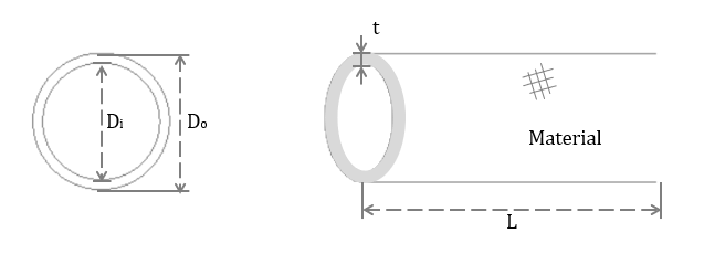
(Figure 1.1)
Diameter (\({\small\displaystyle D}\))
The diameter of a pipe can be divided into inner and outer diameter. The outer diameter is the inner diameter plus twice the thickness of the pipe. Standards for diameter include NPS, DN, and so on. NPS uses inch units, and DN uses mm units. However, the value expressed by NPS or DN does not indicate the actual inner or outer diameter. Therefore, it is necessary to check the value through the chart.
| NPS [inch] | 1/2 | 3/4 | 1 | 11/4 | 11/2 | 2 | 21/2 | 3 | 31/2 | 4 | ... |
| DN [mm] | 15 | 20 | 25 | 32 | 40 | 50 | 65 | 80 | 90 | 100 | ... |
Thickness (\({\small\displaystyle t}\))
Schedule No. is the standard for pipe. The definition of schedule is as follows.
\( \small{\displaystyle \begin{align} Schedule\,No. \quad=\quad 1000\,\frac{P}{S} \tag*{} \end{align} } \)
\({\small\displaystyle P}\) is internal pressure, and \({\small\displaystyle S}\) is the maximum allowable stress of the material. The higher the schedule No, the thicker the thickness. The Schedule No. indicates the classes for the thickness. Pipe thickness should consider various factors such as pressure, allowable stress, temperature, etc. Therefore, we need to calculate the required pipe thickness using other formulas. We will discuss this in another episode.
Material
Pipes are produced in a variety of materials. Also, since each material has different characteristics, we select a suitable material for the process and the cost. We will cover more details about materials in another episode.
2. Design inner diameter of pipe
Assume that fluid flows continuously through a circular pipe completely filling it. How to determine the inner diameter of the pipe? The criterion is “how well the fluid flows?”. We usually check the values for velocity or friction loss to determine it.
The first criterion is the velocity of the fluid. If it is too fast, fluid properties may change, or noise or vibration may occur. Conversely, if it is too slow, it can lead to sedimentation. To prevent these phenomena, we may limit the velocity according to fluid. The equation about the velocity of an incompressible fluid in a circular pipe is as follows.
\( \small{\displaystyle \begin{align} \text{Velocity}\left[\frac{Length}{time}\right] \quad=\quad \frac{\text{Volume rate}\left[\frac{Length^3}{time}\right]}{\text{Area}[Length^2]} \quad=\quad \frac{\dot{V}}{\pi D_i^2/4} \tag{Eq 1.1} \end{align} } \)
The second criterion is friction loss per length. Higher friction loss requires more energy to transport the fluid to the desired point. Among the equations for calculating friction loss, let’s look at the Fanning equation and the Darcy-Weisbach equation.
\( {\small\displaystyle \begin{align} \text{Fanning equation :} \quad h_f \quad&=\quad \frac{\Delta P}{\rho g} \quad=\quad \frac{2f_Fv^2L}{gD} \tag{Eq 1.2} \\[15pt] \text{Darcy-Weisbach equation :} \quad h_f \quad&=\quad \frac{\Delta P}{\rho g} \quad=\quad \frac{1}{2}\,\frac{f_Dv^2L}{gD} \tag{Eq 1.3} \end{align} } \)
Through the two equations, we can know that the friction loss increases as the diameter decreases, and the velocity and friction factor increase. Looking at the two equations above, it seems that the Darcy-Weisbach equation will yield fewer values than the Fanning equation. However, we should get a similar friction loss whichever formula we use. The difference between the two equations is due to the friction factor. Fanning’s friction factor is one-fourth the magnitude of Darcy’s friction factor.
\( \small{\displaystyle \begin{align} f_F \quad=\quad \frac{1}{4}\, f_D \tag{Eq 1.4} \end{align} } \)
We must properly determine permissible friction loss per length. Let’s take a pump system as an example. Below is the equation in Episode 02 of Pump category.
\( \small{\displaystyle \begin{align} h_{TDH} \quad=\quad (h_{sd}\,-\,h_{ss}) \,+\, (h_{fd}\,+\,h_{fs}) \,+\, (h_{vB}\,-\,h_{vA}) \tag{Eq 2.8 in Pump} \end{align} } \)
As the diameter decreases, the friction loss head increases. Therefore, it needs a high total dynamic head to transfer the fluid. And it means the cost of the pump increase. Conversely, if you design the pipe diameter too large to reduce friction loss, the pipe cost will increase significantly.
3. Friction Factor Calculation
For calculating friction loss, we have to know the friction factor. There are two methods for obtaining the friction factor: a method using an equation, and a method using a diagram.
Let’s look at a method using an equation. A representative formula for friction factor is the Colebrook – White equation.
\( {\small\displaystyle \begin{cases} \begin{align} f\quad&=\quad\frac{64}{Re}, &\ \mbox{if }Re\;<\;2,100 \\[15pt] \frac{1}{\sqrt{f}} \quad&=\quad -2log\left(\frac{\varepsilon}{3.7D_h}\;+\;\frac{2.51}{Re\sqrt{f}}\right), &\ \mbox{if }Re\;>\;4,000 \end{align} \end{cases} } \tag{Eq 1.5} \)
When the Reynolds number is less than 2,100, that is, for laminar flow, it can be calculated simply by knowing the Reynolds number. If the Reynolds number is greater than 4,000, the friction factor can be obtained by the trial&error method using the above formula.
A representative diagram for obtaining the friction factor is the Moody diagram.
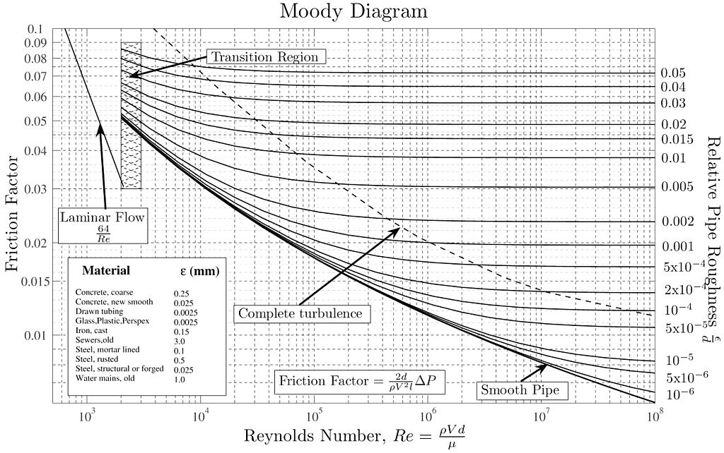
(Figure 1.2) Moody diagram
Donebythesecondlaw at the English Wikipedia, CC BY-SA 3.0 , via Wikimedia Commons
If we know the Reynolds number and relative pipe roughness, we can obtain the friction factor through the diagram. Relative pipe roughness is calculated by dividing the material roughness by the inner diameter. This method is simple. But it may cause some differences depending on the observer.
Both methods described above are friction factors applied to the Darcy-Weisbach equation. If you use another equation or diagram, it is necessary to check which equation applies.
Nomenclature
\({\small\displaystyle D_i}\) : inner diameter
\({\small\displaystyle D_o}\) : outer diameter
\({\small\displaystyle f_D}\) : Darcy-Weisbach friction factor
\({\small\displaystyle f_F}\) : Fanning friction factor
\({\small\displaystyle g}\) : gravitational accerlation
\({\small\displaystyle h_f}\) : friction loss head
\({\small\displaystyle L}\) : length
\({\small\displaystyle P}\) : pressure
\({\small\displaystyle Re}\) : Reynolds number
\({\small\displaystyle S}\) : maximum allowable stress
\({\small\displaystyle v}\) : velocity
\({\small\displaystyle V}\) : volume
\({\small\displaystyle \varepsilon}\) : roughness
\({\small\displaystyle \rho}\) : density
Reference
1. Donebythesecondlaw(2008, July 24). Wikimedia Commons. https://commons.wikimedia.org/wiki/File:Moody_diagram.jpg