Episode 05. Centrifugal Pump - Performance Curve
Summary
In this episode, we discuss the construction of the performance curve for a centrifugal pump. We describe the relationships between total dynamic head, power and flow rate, and efficiency and flow rate, observing their trends. Lastly, we explain how changes in impeller diameter or rotational speed, affect the performance curve.
1. Introduction
When we check pump data, one of the things we encounter is the pump’s performance curve. The specific curve may vary among centrifugal pump manufacturers and models. However, the trend tends to be similar. Let’s describe why the performance curve of the centrifugal pump displays such tendencies, considering the factors mentioned in the previous episodes. In this episode, we explain the performance curve based on impellers with backward–curved blades. In this type, the Euler head decreases as the flow rate increases, but the impeller power remains relatively stable.
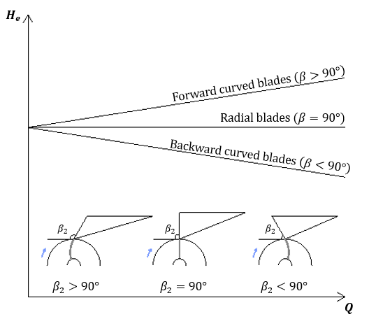
(Figure 5.1)
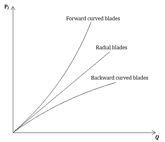
(Figure 5.2)
2. Performance curve of centrifugal pump
Now, let’s look at the performance curve of the centrifugal pump. The performance curve includes three factors based on flow rate :
Total dynamic head, Shaft power, Overall efficiency

(Figure 5.3)
Total dynamic head vs Flow rate
The theoretical head of the fluid from the impeller is the Euler head. However, the pump provides a lower head due to various losses.
One of the losses is flow friction loss. When the cross-sectional area is constant and the flow rate increases, the velocity of the fluid increases. As the velocity of the fluid increases, the friction head also increases according to the following relationship.
\( {\small\displaystyle\begin{align} h_f \quad\propto\quad \frac{v^2}{2g} \tag*{} \end{align} } \)
Especially as the flow rate increases, the influence of the friction head becomes more significant. So, the actual head decreases sharply at high flow rates, resulting in a curve like (Figure 5.3). In (Figure 5.3), the total dynamic head at zero flow rate is called the “shut-off head.”

(Figure 5.4)
Shaft power vs Flow rate
Secondly, let’s examine the relationship between shaft power and flow rate. We know that power is:
\( {\small\displaystyle\begin{align} \mathrm{P} \quad=\quad \rho gQH \tag*{} \end{align} } \)
Looking at the equation, we see that shaft power is affected by flow rate and head. When the head reduction is relatively small compared to the flow rate increase, the shaft power increases as the flow rate rises. Conversely, when the head reduction is greater than the flow rate increase, the shaft power decreases as the flow rate increases. (This tendency is commonly observed in axial flow pumps.)
Shaft power affects fluid temperature. Therefore, in addition to being consumed by various losses, the shaft power is also consumed by temperature rise of the fluid. When the flow rate is low, the temperature rise can be high, resulting in vapor generation and cavitation.
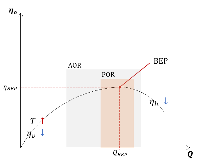
(Figure 5.5)
Efficiency vs Flow rate
Lastly, let’s consider the relationship between efficiency and flow rate. As we learned in Episode 03, overall efficiency can be divided into mechanical, volumetric, and hydraulic efficiency.
\( {\small\displaystyle\begin{align} \eta_o \quad=\quad \eta_m\eta_v\eta_h \tag{Eq 3.7} \end{align} } \)
Mechanical friction occurs in bearings, seals, and other components, regardless of the flow rate. At low flow rates, volumetric efficiency is very low and temperature rise is high, while at high flow rates, hydraulic efficiency is very low. As a result, overall efficiency tends to rise gradually with increasing flow rate until reaching peak efficiency, after which it declines. The point at which efficiency is maximum is referred to as the Best Efficiency Point (BEP) and is usually set to operate near this point (POR).
3. Performance curve depending on impeller diameter or rotational speed
The performance curve of the centrifugal pump described earlier is based on the case where the impeller diameter and the pump’s rotational speed are constant. However, how would the performance curve change if we alter the impeller diameter or the rotational speed? To understand this, we use the affinity laws.
\( {\small\displaystyle\begin{align} \frac{Q_1}{Q_2} \quad&=\quad \left(\frac{D_1}{D_2}\right) \left(\frac{N_1}{N_2}\right) \tag{Eq 5.1} \\[15pt] \frac{H_1}{H_2} \quad&=\quad \left(\frac{D_1}{D_2}\right)^2 \left(\frac{N_1}{N_2}\right)^2 \tag{Eq 5.2} \\[15pt] \frac{P_1}{P_2} \quad&=\quad \left(\frac{D_1}{D_2}\right)^3 \left(\frac{N_1}{N_2}\right)^3 \tag{Eq 5.3} \end{align} } \)
Changing the impeller diameter at a constant rotational speed, we get:
\( {\small\displaystyle\begin{align} \frac{Q_1}{Q_2} \,=\, \frac{D_1}{D_2},\qquad \frac{H_1}{H_2} \,=\, \left(\frac{D_1}{D_2}\right)^2,\qquad \frac{\mathrm{P}_1}{\mathrm{P}_2} \,=\, \left(\frac{D_1}{D_2}\right)^3 \tag{Eq 5.4} \end{align} } \)
On the other hand, changing the rotational speed at a constant impeller diameter, we get:
\( {\small\displaystyle\begin{align} \frac{Q_1}{Q_2} \,=\, \frac{N_1}{N_2},\qquad \frac{H_1}{H_2} \,=\, \left(\frac{N_1}{N_2}\right)^2,\qquad \frac{\mathrm{P}_1}{\mathrm{P}_2} \,=\, \left(\frac{N_1}{N_2}\right)^3 \tag{Eq 5.5} \end{align} } \)
Using these equations, we can plot the performance curves of the centrifugal pump for each case as shown in (Figure 5.6) and (Figure 5.7). The overall efficiency is assumed to be similar.
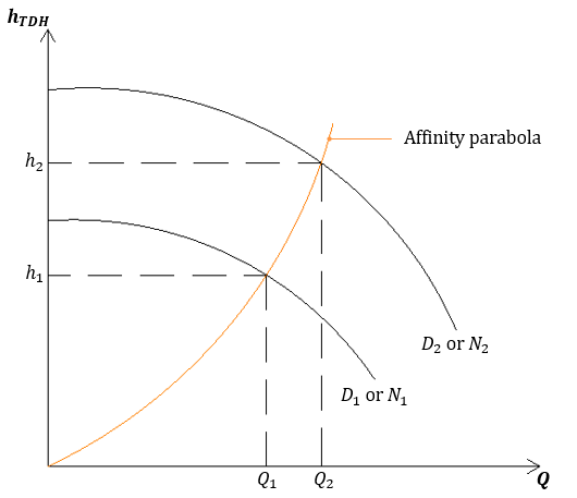
(Figure 5.6)
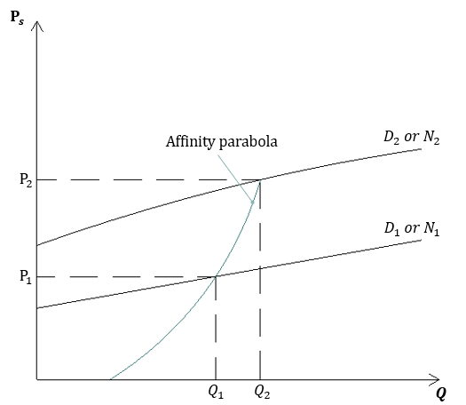
(Figure 5.7)
Affinity laws enable us to predict pump performance in each scenario. However, it’s essential to be cautious as accuracy may decrease. (especially, changes in impeller diameter) Some manufacturers also provide pump performance curves for each specific scenario.
Nomenclature
\({\small\displaystyle \text{AOR}}\) : allowable operating range
\({\small\displaystyle D}\) : diameter
\({\small\displaystyle g}\) : gravitational accerleration
\({\small\displaystyle H}\) : head
\({\small\displaystyle h_f}\) : friction head
\({\small\displaystyle h_{TDH}}\) : total dynamic head
\({\small\displaystyle N}\) : rotational speed
\({\small\displaystyle \mathrm{P}}\) : power
\({\small\displaystyle \mathrm{P}_s}\) : shaft power
\({\small\displaystyle \text{POR}}\) : preferred operating range
\({\small\displaystyle Q}\) : flow rate
\({\small\displaystyle v}\) : velocity
\({\small\displaystyle \rho}\) : density
\({\small\displaystyle \eta_h}\) : hydraulic efficiency
\({\small\displaystyle \eta_m}\) : mechanical efficiency
\({\small\displaystyle \eta_o}\) : overall efficiency
\({\small\displaystyle \eta_v}\) : volumetric efficiency